
Overview
I recently spent some time near Huntington Lake- one of the more interesting sailing lakes in California. Lashing a GPS to the front of the boat was an enlightening way to look at the spatial and angular trends in the amount of speed I could get out of this boat. With 218 sq. feet of sail, and only 320 lbs of displacement (i.e. the boat's weight) - the Hobie 16 is an exciting 2 person boat for light to medium winds. With my regular crew absent we did not use a trapeze and thus were only able to get the boat to about 11 knots (6 m/s).
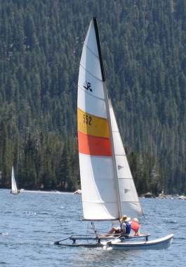 Two short excursions (approx. 5 miles each) were measured with a Garmin GPS 12, which was set to record a track point every 5 seconds. With an open horizon, and such a short tracking interval it was possible to accurately map out changes in velocity and direction over the duration of the excursions.
GRASS was used to extract line segment start and end nodes, calculate line segment length, and assign a velocity to each line segment. These data were dumped to CSV file for analysis in R. Simple plots of velocity vs. bearing from east were created. All code and GPS logs (see attached files) are included on this page. These examples demonstrate several simple GIS and plotting techniques which can be performed in GRASS & R with very few keystrokes.
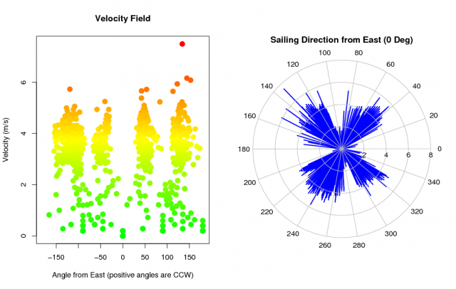
Figure: Boat speed vs. angle to the wind
Huntington Lake Bathymetry
Contours below lake level were digitized off a USGS topographic map, and an estimated elevation surface was interpolated with the RST algorithm as implemented in GRASS (v.surf.rst). This algorithm can use either iso-lines (contours) or spot (point) elevations for the interpolation. Commands used included v.digit, v.to.rast, v.surf.rst, v.type, and r.mapcalc
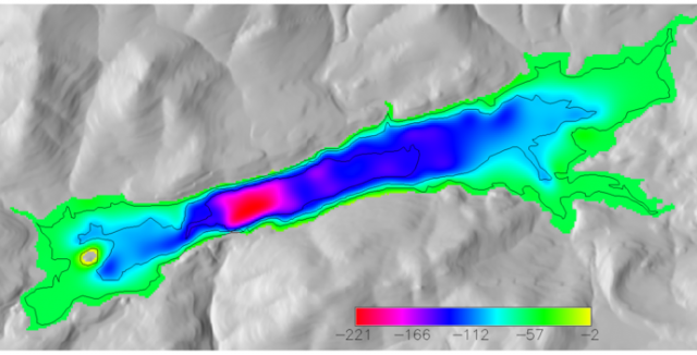
Figure: Huntington Lake Estimated Bathymetry Units are feet below lake level
Data dump and preprocessing with AWK
## download track data as points with gpstrans
gpstrans -dt > output.raw

# trim top couple of garbage lines off with text editor...

# convert into GRASS line segments with AWK
awk '
BEGIN{print "VERTI:"; n = 0}
{
vertex = $6" "$7
if(  (n > 0 && n < 3) ) {print "L 2\n"old_vertex"\n"vertex}
else if(n >2 ) {print "L 2\n"old_vertex"\n"vertex}
old_vertex = vertex; n++
}
' output.raw > output.ascii
GIS processing in GRASS
# need to pre-make the hobie.ascii file first!
# these were generated with a combination of gpstrans and awk

# this is the prefix i.e. 'hobie1'
infile=$1

## import and make table
v.in.ascii --o in=$infile.ascii out=$infile format=standard


## add cat to line features
v.category in=$infile out=htemp option=add type=line

## rename, and overwrite the original vector
g.remove vect=$infile
g.rename vect=htemp,$infile

v.db.addtable map=$infile columns="cat int, len double, velocity double, start_x double, start_y double, end_x double, end_y double"

## upload data by cat -- for each line segment
# v.to.db map=$infile column=cat option=cat
v.to.db map=$infile column=len option=length
v.to.db map=$infile column=start_x,start_y option=start
v.to.db map=$infile column=end_x,end_y option=end

## calculate velocity in m/s (assuming 5 second interval)
echo "update $infile set velocity = len / 5" | db.execute

db.select $infile fs="," > $infile.csv
Bearing calculations and plotting ideas in R
# read in some data:
# these were dumped from GRASS
x <- read.csv('hobie1.csv')
y <- read.csv('hobie2.csv')

# some diagnostics:
plot(cumsum(x$len), type='l')
plot(cumsum(y$len), type='l')
plot( density(x$velocity[x$velocity > 1]))
plot( density(y$velocity[y$velocity > 1]))

# compute angle from x-axis, with quadrant correction
# this is the same as atan(dx/dy) + quadrant test
# i.e. this is the angle (neg = CW / pos = CCW) from East (E = 0 Deg)
#
# we can check this with a combination of d.grid and d.vect for
# specific lines
# d.grid -t -b size=10 origin=306791,4123865
# d.vect hobie2 disp=shape,cat,dir cat=120-130
# matches y[122,]  ---> angle = 135 Deg
#

dx <- with(x, (end_x - start_x))
dy <- with(x, (end_y - start_y))
x$angle  <- atan2(dy, dx) * 180/pi

dx <- with(y, (end_x - start_x))
dy <- with(y, (end_y - start_y))
y$angle  <- atan2(dy, dx) * 180/pi

# combine into a single df
# remove bogus values
z <- rbind(x,y)
z <- na.omit(z)

# load required packages
library(plotrix)

## angle vs velocity on linear plot
par(mfcol=c(1,2))

plot(velocity ~ angle, data=z, xlim=c(-180,180), xlab="Angle from East (positive angles are CCW)",
ylab="Velocity (m/s)", main="Velocity Field", col=color.scale(velocity,c(0,1,1),c(1,1,0),0), pch=16, cex=1.5)

## polar plot:
polar.plot(z$velocity, z$angle ,main="Sailing Direction from East (0 Deg)", line.col='blue', lwd=2)
Attachments:
