
Higher Order Transformations
... Continuing from the initial example session in R ...
An affine transformation is based on a linear mapping between two coordinate-spaces. Testing for non-linearity (i.e. higher order model terms) can be a useful diagnostic in choosing the simpler affine transform.
Compute the difference between the good and bad coordinates
## compute vector difference and save back to original data frame:
c$sqdiff <- with(c, sqrt((nx-x)^2 + (ny-y)^2))
Generate two linear models:
## generate simple model
l.simple <- lm(sqdiff ~ nx + ny, data=c)
## model with higher order terms (up to 3rd-order):
## note to self: poly() computes orthagonal polynomials
l.poly <- lm(sqdiff ~ poly(nx, 3) + poly(ny, 3), data=c)


## summarize the complex model:
summary(l.poly)
Coefficients:
             Estimate Std. Error t value Pr(>|t|)
(Intercept)    302.38       3.97  76.174  < 2e-16 ***

poly(nx, 3)1  1091.17      35.82  30.466  < 2e-16 ***
poly(nx, 3)2   165.59      32.78   5.051 1.71e-05 ***
poly(nx, 3)3   -51.21      28.74  -1.782   0.0843 .

poly(ny, 3)1   417.35      31.97  13.056 2.30e-14 ***
poly(ny, 3)2   -18.50      30.04  -0.616   0.5425
poly(ny, 3)3    19.41      35.49   0.547   0.5882

---
Signif. codes:  0 ‘***’ 0.001 ‘**’ 0.01 ‘*’ 0.05 ‘.’ 0.1 ‘ ’ 1
Is one model significantly better than the other?
## check via RMSE:
## simple model
sqrt( mean((fitted(l.simple) - c$sqdiff)^2) )
36.54747


## model with 3rd-order polynomial
sqrt( mean((fitted(l.poly) - c$sqdiff)^2) )
22.45530


## the anova function can compare nested models:
anova(l.simple, l.poly)
Analysis of Variance Table

Model 1: sqdiff ~ nx + ny
Model 2: sqdiff ~ poly(nx, 3) + poly(ny, 3)
  Res.Df   RSS Df Sum of Sq      F    Pr(>F)
1     36 52093
2     32 19665  4     32428 13.192 1.865e-06 ***
---
Signif. codes:  0 ‘***’ 0.001 ‘**’ 0.01 ‘*’ 0.05 ‘.’ 0.1 ‘ ’ 1
Check visually:
## re-make grid of points to predict on: ## and save two versions to 'stack-up' x <- seq(-2080000, -2040000, by=1000) y <- seq(-20000, 5000, by=2000) d.simple <- expand.grid(x=x, y=y) d.poly <- expand.grid(x=x, y=y) ## and predict the trend in differences: d.simple$diff <- predict(l.simple, data.frame(nx=d$x, ny=d$y)) d.poly$diff <- predict(l.poly, data.frame(nx=d$x, ny=d$y)) ## stack for grouped plotting library(lattice) library(RColorBrewer) d.combined <- make.groups(simple=d.simple, poly=d.poly) ## plot: wireframe(diff ~ x * y | which, data=d.combined, scales=list(arrows=TRUE), drape=TRUE, col.regions=brewer.pal(n=9, name='Oranges'), cuts=8, col='white')
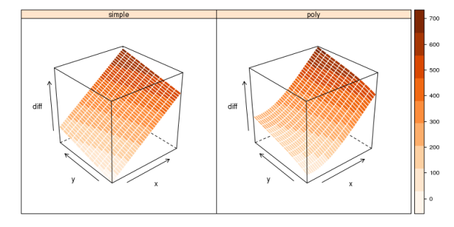
Testing for linearity: Two visualizations of the deviance between coordinates positions, at the control point locations.
Conclusions:
It seems that a second order term was only warranted along the x-direction. The more complex model based on 3rd-order polynomials results in a significantly lower RMSE (about 10 meters lower), and is shown to be a better descriptor of variance in the test of nested models.
At the map scale in which the corrected data will be presented, the extra accuracy suggested by the more complex model (coordinate transformation function) is negligible. This allows for the simpler model, which can be directly used by the convenient ST_Affine() function in PostGIS for the heavy-lifting.
