Numerical Integration/Differentiation in R: FTIR Spectra
Feb 23, 2010 metroadminStumbled upon an excellent example of how to perform numerical integration in R. Below is an example of piece-wise linear and spline fits to FTIR data, and the resulting computed area under the curve. With a high density of points, it seems like the linear approximation is most efficient and sufficiently accurate. With very large sequences, it may be necessary to adjust the value passed to the subdivisions argument of integrate(). Strangely, larger values seem to solve problems encountered with large datasets...

FIgure: FTIR Spectra Integration
Implementation
# numerical integration in R
# example based on: http://tolstoy.newcastle.edu.au/R/help/04/10/6138.html

# sample data: FTIR spectra
x <- read.csv(url('http://casoilresource.lawr.ucdavis.edu/drupal/files/fresh_li_material.CSV'), header=FALSE)[100:400,]
names(x) <- c('wavenumber','intensity')

# fit a piece-wise linear function
fx.linear <- approxfun(x$wavenumber, x$intensity)

# integrate this function, over the original limits of x
Fx.linear <- integrate(fx.linear, min(x$wavenumber), max(x$wavenumber))

# fit a smooth spline, and return a function describing it
fx.spline <- splinefun(x$wavenumber, x$intensity)

# integrate this function, over the original limits of x
Fx.spline <- integrate(fx.spline, min(x$wavenumber), max(x$wavenumber))

# visual check, linear and spline fits shifted up for clarity
par(mar=c(0,0,0,0))
plot(x, type = "p", las=1, axes=FALSE, cex=0.5, ylim=c(0,0.12))
lines(x$wavenumber, fx.linear(x$wavenumber) + 0.01, col=2)
lines(x$wavenumber, fx.spline(x$wavenumber) + 0.02, col=3)
grid(nx=10, col=grey(0.5))
legend(x=615, y=0.11, legend=c('original','linear','spline'), col=1:3, pch=c(1,NA,NA), lty=c(NA, 1, 1), bg='white')

# results are pretty close
data.frame(method=c('linear', 'spline'), area=c(Fx.linear$value, Fx.spline$value), error=c(Fx.linear$abs.error,Fx.spline$abs.error))

  method     area        error
1 linear 27.71536 0.0005727738
2 spline 27.71527 0.0030796529
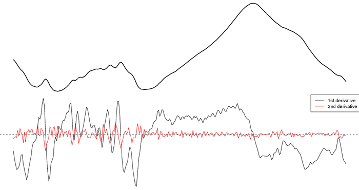
splinefun() can also compute derivatives
par(mar=c(0,0,0,0), mfcol=c(2,1))
plot(x, type = "l", lwd=2, axes=FALSE)
grid(nx=10, col=grey(0.5))
plot(x$wavenumber, fx.spline(x$wavenumber, deriv=1), type='l', axes=FALSE)
lines(x$wavenumber, fx.spline(x$wavenumber, deriv=2), col='red')
grid(nx=10, col=grey(0.5))
abline(h=0, lty=2)
legend('topright', legend=c('1st derivative','2nd derivative'), lty=1, col=1:2, bg='white')

Figure: Numerical Estimation of Derivatives
Attachment:
Links:
Additional Example Using Lattice Graphics
R: advanced statistical package
Plotting XRD (X-Ray Diffraction) Data
Software
- General Purpose Programming with Scripting Languages
- LaTeX Tips and Tricks
- PostGIS: Spatially enabled Relational Database Sytem
- PROJ: forward and reverse geographic projections
- GDAL and OGR: geodata conversion and re-projection tools
- R: advanced statistical package
- Access Data Stored in a Postgresql Database
- Additive Time Series Decomposition in R: Soil Moisture and Temperature Data
- Aggregating SSURGO Data in R
- Cluster Analysis 1: finding groups in a randomly generated 2-dimensional dataset
- Color Functions
- Comparison of Slope and Intercept Terms for Multi-Level Model
- Comparison of Slope and Intercept Terms for Multi-Level Model II: Using Contrasts
- Creating a Custom Panel Function (R - Lattice Graphics)
- Customized Scatterplot Ideas
- Estimating Missing Data with aregImpute() {R}
- Exploration of Multivariate Data
- Interactive 3D plots with the rgl package
- Making Soil Property vs. Depth Plots
- Numerical Integration/Differentiation in R: FTIR Spectra
- Plotting XRD (X-Ray Diffraction) Data
- Using lm() and predict() to apply a standard curve to Analytical Data
- Working with Spatial Data
- Comparison of PSA Results: Pipette vs. Laser Granulometer
- GRASS GIS: raster, vector, and imagery analysis
- Generic Mapping Tools: high quality map production

