Home Software R: advanced statistical package Working with Spatial Data Ordinary Kriging Example: GRASS-R Bindings

Ordinary Kriging Example: GRASS-R Bindings

Update: 2012-02-13
Many of the examples used in this demonstration are now somewhat dated, probably inefficient, and in need of revision. I'll spend some time on an updated version for the GRASS wiki soon.

Overview:
A simple example of how to use GRASS+R to perform interpolation with ordinary kriging, using data from the spearfish sample dataset. This example makes use of the gstat library for R.

Helpful References:

Issaks, E.H. & Srivastava, R.M. An Introduction to Applied Geostatistics Oxford University Press, 1989
GSTAT Manual
GSTAT Examples

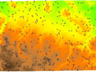
Elevation Data and Sample Points: 300 randomly placed points where elevation data was sampled.

Data Prep:
As a contrived example, we will generate 300 random points within the current region, and sample an elevation raster at each of these points.


# set region:
g.region rast=elevation.dem
# extract some random points from an elevation dataset
v.random out=rs n=300
# create attribute table:
v.db.addtable map=rs columns="elev double"
# extract raster data at points
v.what.rast vect=rs rast=elevation.dem column=elev
# simple display:
d.rast elevation.dem
d.vect rs size=4
# start R
R
X

Load GRASS Data into R:
Remember that you will need to install these R packages onto your computer.


##load libraries
library(gstat)
library(spgrass6)
## read in vector dataset from above
G <- gmeta6()
x.has.na <- readVECT6('rs')
# remove records with NA
x <- x.has.na[-which(is.na(x.has.na@data$elev)),]
## create a grid wihch will define the interpolation
## note that it is based on the current GRASS region settings
grd <- gmeta2grd()
## make a new grid of (1)s
## be sure to use original data's proj data...
## doesn't work with the stuff stored in G...
new_data <- SpatialGridDataFrame(grd, data=data.frame(k=rep(1,G$cols*G$rows)), proj4string=CRS(x@proj4string@projargs))
## optionally we can use another raster of 1's as our interpolation mask
mask <- as(readRAST6("rushmore"), "SpatialPixelsDataFrame")
## need to manually set the coordinate system information:
mask@proj4string <- x@proj4string
## this new object could then be used in the 'newdata' argument to predict(), i.e.
## x.pred_OK <- predict(g, id='elev', newdata=mask)
X

Variogram Modeling:
A very simple example, using default parameters for a non-directional variogram is presented below. Modeling the variogram for an actual spatial problem requires knowlege of both your dataset (distribution, collection methods, etc.), the natural processes involved (stationarity vs. anisotropy ?), and a bit about the assumptions of geostatistics.


## init our gstat object, with the model formula
## note that coordinates are auto-identified from the GRASS object
g <- gstat(id="elev", formula=elev ~ 1, data=x)
## view a variogram with specified parameters
plot(variogram(g, width=250, cutoff=10000, map=FALSE))
## optionally make a variogram map, and plot semi-variance for 10-point pairs or greater:
plot(variogram(g, width=250, cutoff=10000, map=TRUE), threshold=10)
## fit a linear variogram model- as this looks appropriate
## ... using default parameters
v.fit <- fit.variogram(variogram(g) ,vgm(model="Lin") )
plot(variogram(g, width=250, cutoff=10000, map=FALSE), model=v.fit)
## update gstat object with fitted variogram model
g <- gstat(g, id="elev", model=v.fit )
X

Variogram and Fit Model: A Linear variogram model was fit to the elevation data.
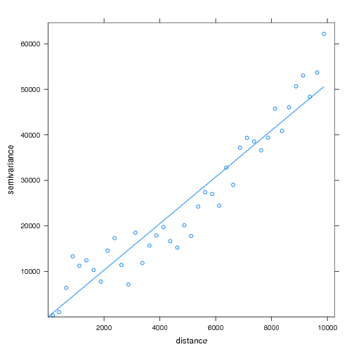
Variogram and Fit Model: A Linear variogram model was fit to the elevation data.

Interpolation by Ordinary Kriging:
The prediction is done for every instance of a '1' in the object passed to the newdata= argument.


## interpolate with ord. kriging
x.pred_OK <- predict(g, id='elev', newdata=new_data)
X

Send Results Back to GRASS:


## write raster back to GRASS: interpolation and kriging variance:
## system('g.remove rast=elev.ok')
writeRAST6(x.pred_OK, 'elev.ok', zcol='elev.pred')
writeRAST6(x.pred_OK, 'elev.ok_var', zcol='elev.var')
## quit:
q()
X

Viewing Results in GRASS:


# reset colors to match original data:
r.colors map=elev.ok rast=elevation.dem
# give the kriging variance a grey color map
r.colors map=elev.ok_var color=rules <<EOF
0% white
100% black
EOF
#
# display the kriged interpolation, with intensity | saturation based on variance
d.his s=elev.ok_var h=elev.ok
# optional method:
# d.his i=elev.ok_var h=elev.ok
d.vect rs size=4
X

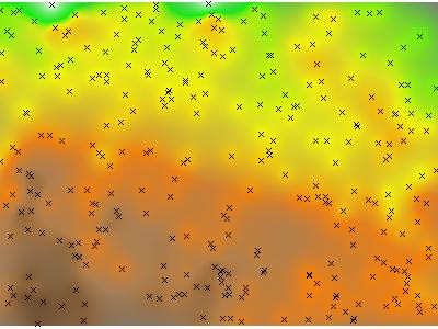
Interpolated Elevation Data via Ordinary Kriging: Hue is interpolated elevation value, saturation is based on the kriging variance.

Simple Comparison with RST:
RST (regularized splines with tension) and OK (ordinary kriging) are two common interpolation methods. Computing the RMSE (root-mean-square-error) between the interpolated raster and the original raster provides a simple quantitative measure of how well the interpolation performed, at least in terms mean magnitude of error. A spatial description of interpolation error can be generated by subtracting the new raster from the original. Note that the steps involve cell-wise computation of the square-error (SE), region-wise computation of the mean-square-error (MSE); the square root of MSE gives the root-mean-square-error or RMSE.


#
# compare with RST - tension of 60, same points
#
v.surf.rst in=rs elev=elev.rst zcol=elev tension=60
r.colors map=elev.rst rast=elevation.dem
# compute SE between kriged map and original
r.mapcalc "d = (elev.ok - elevation.dem)^2 "
r.colors map=d color=rainbow
d.rast d
d.vect rs size=4
# compute SE between RST map and original
r.mapcalc "d2 = (elev.rst - elevation.dem)^2"
r.colors map=d2 color=rainbow
d.rast d2
d.vect rs size=4
#
# compare results:
#
# compute RMSE for OK [sqrt(MSE)]
r.univar d
# compute RMSE for RST [sqrt(MSE)]
r.univar d2
# see table below:
X

Root-mean-square-error Comparison:
Looks like the RSME are pretty close...

Method	OK	RST
RMSE	61 meters	64 meters