
Premise
Simple demonstration of working with time-series data collected from Decagon Devices soil moisture and temperature sensors. These sensors were installed in a potted plant, that was semi-regularly watered, and data were collected for about 80 days on an hourly basis. Several basic operations in Rare demonstrated:
- reading raw data in CSV format
- converting date-time values to R's date-time format
- applying a calibration curve to raw sensor values
- initialization of R time series objects
- seasonal decomposition of additive time series (trend extraction)
- plotting of decomposed time series, ACF, and cross-ACF
Process the raw sensor values with standard calibrations
## data from office plant: in potting soil
# raw data dump -- need to convert datetime + values:
x1 <- read.csv('office_plant_2.csv', head=FALSE)

# datetime is seconds from jan 1st 2000
t_0 <- as.POSIXlt(strptime('2000-01-01 00:00:00', format='%Y-%m-%d %H:%M:%S'))

# calibration for potting soil
raw_to_vwc <- function(d) {vwc <- (d * 0.00119) - 0.401 ; vwc }

# calibration for deg C
raw_to_temp <- function(d) {t <- log( (4095/d) - 1 ) ; t_c <-  25.02 + t * (-22.84 + t * (1.532 + (-0.08372 * t))) ; t_c}

# convert values
y1 <- data.frame(date=t_0 + x1$V1, m=raw_to_vwc(x1$V2), t=raw_to_temp(x1$V5))

# make a nice time axis
d.range <- range(y1$date)
d.list <- seq(d.range[1], d.range[2], by='week')

# note that there are several tricks here:
# stacking two plots that share an axis
# customized x-axis
# and manually adding a title with mtext()
par(mar = c(0.5, 4, 0, 1), oma = c(3, 0, 4, 0), mfcol = c(2,1))
plot(m ~ date, data=y1, type='l', ylab='VWC (EC-5 Sensor)', xaxt='n', las=2, cex.axis=0.75)
plot(t ~ date, data=y1, type='l', ylab='Deg. C (EC-T Sensor)', xaxt='n', las=2, cex.axis=0.75)
axis.POSIXct(at=d.list, side=1, format="%b-%d", cex.axis=0.75)
mtext('Potted Plant Experiment', outer=TRUE, line=2, font=2)

# save copy of raw data
dev.copy2pdf(file='raw_data.pdf')
Decompose each time series into additive components
# look at components of time series:
# we recorded measurements once and hour, so lets consider these data a on a daily-cycle
temp.ts <- ts(y1$t, freq=24)
vwc.ts <- ts(y1$m, freq=24)

# decompose additive time series with STL
# (Seasonal Decomposition of Time Series by Loess)
temp.stl <- stl(temp.ts, s.window=24)
vwc.stl <- stl(vwc.ts, s.window=24)

# these are referenced by day, so we need a new index for
# plotting meaningful dates on the x-axis
# generate the difference in days, from the first observations, at each date label
date.day_idx <- as.numeric((d.list - d.range[1]) / 60 / 60 / 24)

# note special syntax
par(mar = c(0, 4, 0, 3), oma = c(5, 0, 4, 0), mfcol = c(4,1), xaxt='n')
plot(temp.stl , main='Temperature (deg C)')
mtext(at=date.day_idx, text=format(d.list, "%b-%d"), side=1, cex=0.75)
dev.copy2pdf(file='temperature-ts_plot.pdf')

# note special syntax
par(mar = c(0, 4, 0, 3), oma = c(5, 0, 4, 0), mfcol = c(4,1), xaxt='n')
plot(vwc.stl , main='Volumetric Water Content')
mtext(at=date.day_idx, text=format(d.list, "%b-%d"), side=1, cex=0.75)
dev.copy2pdf(file='vwc-ts_plot.pdf')
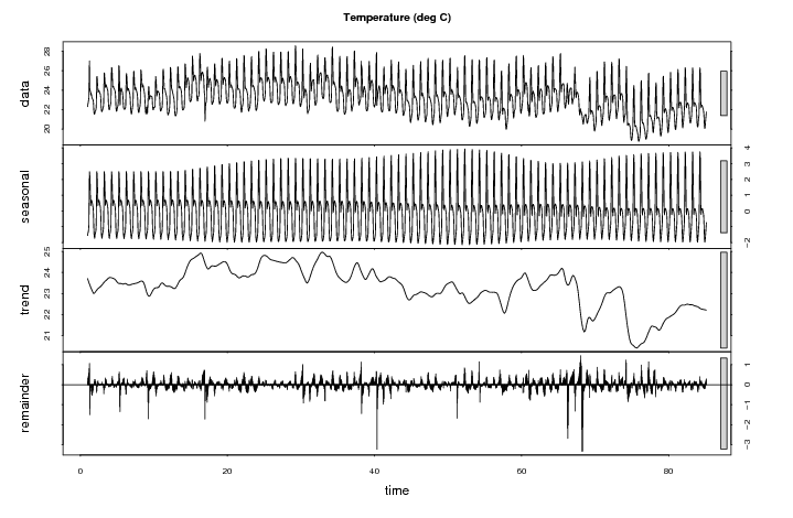
Additive Time Series Decomposition: Temperature
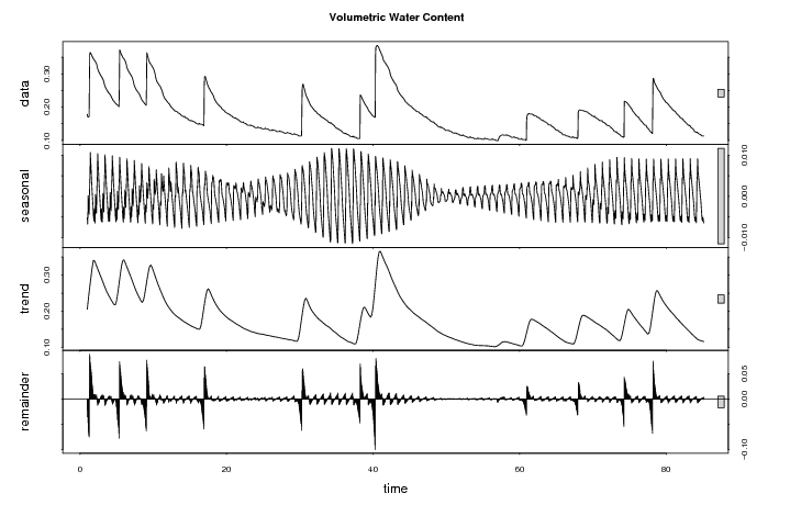
Additive Time Series Decomposition: Volumetric Water Content
Auto-Correlation Function (ACF)
# look at ACF: ind. time series, and cross-ACF
acf( ts.union(temp.ts, vwc.ts) )

# extract seasonal components from each sensor, union, and plot together
temp_vwc.ts <- ts.union(Temperature=temp.stl$time.series[,1], VWC=vwc.stl$time.series[,1])
plot(temp_vwc.ts, main='Seasonal Components', mar.multi= c(1, 5.1, 1, 1))
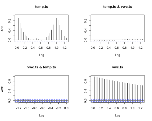
Soil Moisture and Temperature ACF: Auto-correlation function of each time series, and cross-ACF.
Interesting Results
Variation in temperature with time dominated by diurnal fluctuations superposed over underlying fluctuations caused by building heating/cooling system. The magnitude of the diurnal cycle appears to be related to the moisture content- as expected due to high heat capacity of water. Diurnal variation in moisture values appears to account for less than < 2% absolute change in volumetric water content.
Attachment:
Links:
Access Data Stored in a Postgresql Database
R: advanced statistical package
