
Using lm() and predict() to apply a standard curve to Analytical Data
Load input data (see attached files at bottom of this page)
#first the sample data
#note that field sep might be different based on pre-formatting
cn <- read.table("deb_pinn_C_N-raw.final.txt", sep=" ", header=TRUE)

#then the standards:
cn_std <- read.table("deb_pinn_C_N-standards.final.txt", sep="\t", header=TRUE)

# comput simple linear models from standards
# "mg_nitrogen as modeled by area under curve"
lm.N <- lm(mg_N ~ area_N, data=cn_std)
lm.C <- lm(mg_C ~ area_C, data=cn_std)

# check std curve stats:
summary(lm.N)
 Multiple R-Squared: 0.9999,     Adjusted R-squared: 0.9999
summary(lm.C)
 Multiple R-Squared:     1,      Adjusted R-squared:     1
Apply the standard curve to the raw measurements
# note that the predict method is looking for column names that where originally
# used in the creation of the lm object
# i.e. area_N for lm.N  and area_C for lm.C
# therefore it is possible to pass the original data matrix with both
# values to predict(), while specifiying the lm object
cn$mg_N <- predict(lm.N, cn)
cn$mg_C <- predict(lm.C, cn)
Merge sample mass to calculate percent C/N by mass
#read in the initial mass data, note that by default string data will be read in as a factor
# i.e. factors are like treatments, and this data type will not work in some functions
cn.mass <- read.table("all_samples.masses.txt", header=TRUE, sep="\t")

#take a look at how the mass data was read in by read.table()
str(cn.mass)
'data.frame':   75 obs. of  5 variables:
 $ id         : <b>Factor</b> w/ 26 levels</b> "004K","007K",..: 15 16 17 18 19 20 21 22 23 24 ...
 $ pedon_id   : <b>Factor</b> w/ 18 levels "004K","007K",..: 15 15 15 18 18 18 17 17 17 16 ...
 $ horizon_num: int  2 5 7 2 4 6 2 4 5 2 ...
 $ sample_id  : <b>Factor</b> w/ 75 levels "A1","A10","A11",..: 23 24 14 15 16 25 29 30 31 32 ...
 $ sample_mg  : num  24.6 27.5 33.3 25.9 25.8 ...


# use the merge() function to join the two dataframes based on the cell_id column
#merge() does not work with columns of type "level"
# convert them to characters in upper case, and append them to the original dataframe:
# note that merge is case sensitive !!!
cn$cell_id <- toupper(as.character(cn$sample_id))
cn.mass$cell_id <- toupper(as.character(cn.mass$sample_id))

#only keep our pedon data, leave behind the checks
cn.complete <- merge(x=cn, y=cn.mass, by.x="cell_id", by.y="cell_id", sort=FALSE, all.y=TRUE)

##calculate percent N and C, appending to the cn.complete dataframe
cn.complete$pct_N <- (cn.complete$mg_N / cn.complete$sample_mg) * 100
cn.complete$pct_C <- (cn.complete$mg_C / cn.complete$sample_mg) * 100

#look at the results:
str(cn.complete)
'data.frame':   75 obs. of  13 variables:
 $ cell_id    : chr  "B8" "B9" "B10" "B11" ...
 $ sample_id.x: Factor w/ 81 levels "A1","A10","A11",..: 24 25 15 16 17 26 30 31 32 33 ...
 $ area_N     : num  2225431  208028  341264 1377688  168328 ...
 $ area_C     : num  85307240  8296664 14624760 50879560  6690868 ...
 $ mg_N       : num  0.09261 0.01096 0.01635 0.05830 0.00935 ...
 $ mg_C       : num  1.2609 0.1204 0.2141 0.7510 0.0967 ...
 $ id         : Factor w/ 26 levels "004K","007K",..: 15 16 17 18 19 20 21 22 23 24 ...
 $ pedon_id   : Factor w/ 18 levels "004K","007K",..: 15 15 15 18 18 18 17 17 17 16 ...
 $ horizon_num: int  2 5 7 2 4 6 2 4 5 2 ...
 $ sample_id.y: Factor w/ 75 levels "A1","A10","A11",..: 23 24 14 15 16 25 29 30 31 32 ...
 $ sample_mg  : num  24.6 27.5 33.3 25.9 25.8 ...
 $ pct_N      : num  0.3759 0.0398 0.0491 0.2254 0.0363 ...
 $ pct_C      : num  5.117 0.438 0.643 2.903 0.375 ...

#save the data for further processing:
write.table(cn.complete, file="cn.complete.table", col.names=TRUE, row.names=FALSE)
Measure the accuracy of the sensor in the machine with simple correlation
### get a measure of how accurate the sensor was, based on our checks:
#just the first 5 columns, in case there is extra
cn.checks <- cn[c(13,26,39,52,65,78),][1:5]

#make a list of the mg of ACE in each check
checks.mg_ACE <- c(0.798, 1.588, 1.288, 1.574, 1.338, 1.191)

#make a column of the REAL mg_N based on the percent N in ACE
cn.checks$real_mg_N  <- checks.mg_ACE * 0.104

#make a column of the REAL mg_C based on the percent C in ACE
cn.checks$real_mg_C  <- checks.mg_ACE * 0.711

# check with cor()
Create a mutli-figure diagnostic plot
layout(mat=matrix(c(1, 4, 2, 3), nc = 2, nr = 2), width=c(1,1), height=c(1,2))
#first the std curves
par(mar = c(4,4,2,2))

#Nitrogen
plot(mg_N ~ area_N, data=cn_std, xlab="Area Counts", ylab="mg", main="Std Curve for N", cex=0.7, pch=16, cex.axis=0.6)
rug(cn$area_N, ticksize=0.02, col="gray")
rug(cn$mg_N, ticksize=0.02, col="gray", side=2)
abline(lm.N, col="gray", lty=2)
points(cn$area_N, cn$mg_N, col="blue", cex=0.2, pch=16)

#Carbon
plot(mg_C ~ area_C, data=cn_std, xlab="Area Counts", ylab="mg", main="Std Curve for C", cex=0.7, pch=16, cex.axis=0.6)
rug(cn$area_C, ticksize=0.02, col="gray")
rug(cn$mg_C, ticksize=0.02, col="gray", side=2)
abline(lm.C, col="gray", lty=2)
points(cn$area_C, cn$mg_C, col="blue", cex=0.2, pch=16)
#possible problems
points(cn$area_C[which(cn$area_C > 1.0e+08)], cn$mg_C[which(cn$area_C > 1.0e+08)] , col="red")

#sample plot of carbon distributions within each pedon:
#note that las=2 makes axis labels perpendicular to axis
par(mar = c(7,4,4,2))

#boxplot illustrating the within-pedon variation of Carbon
boxplot(cn.complete$pct_C ~ cn.complete$pedon_id , cex.axis=0.6, boxwex=0.2, las=2, main="Percent Total Carbon", ylab="% C", xlab="Pedon ID", cex=0.4)

#boxplot illustrating the within-pedon variation of Nitrogen
boxplot(cn.complete$pct_N ~ cn.complete$pedon_id , cex.axis=0.6, boxwex=0.2, las=2, main="Percent Total Nitrogen", ylab="% N", xlab="Pedon ID", cex=0.4)
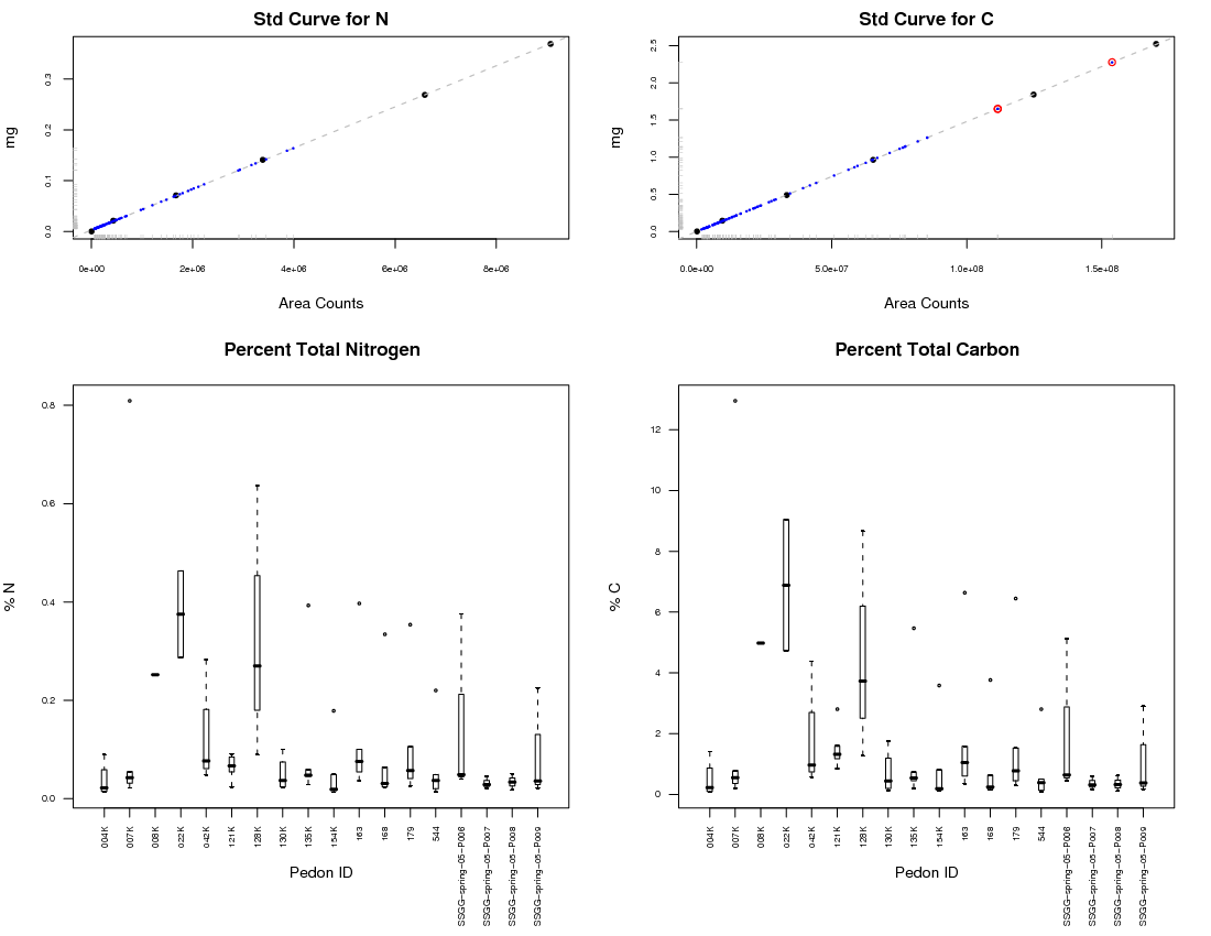
R: Multi-figure plot of Carlo-Erba Data
Attachments:
deb_pinn_C_N-raw.final_.txt
deb_pinn_C_N-standards.final_.txt
all_samples.masses.txt
