
Overview:
Simple application of spatial point-process models to spread patterns after some backyard target practice. Note that only a cereal box and 2 sheets of graph paper were injured in this exercise. Data files are attached at the bottom of this page; all distance units are in cm.
A simple experiment was conducted, solely for the purpose of collecting semi-random coordinates on a plane, where a target was hit with 21 shots from a distance of 15 and 30 feet. The ppm() function (spatstat package) in R was used to create point density maps, along with a statistical description of the likelihood of where each target would be hit were the experiment to be conducted again (via point-process modeling). While normally used to model the occurrence of natural phenomena or biological entities, point-process models can be used to analyze one's relative accuracy at set target distances. One more way in which remote sensing or GIS techniques can be applied to smaller, non-georeferenced coordinate systems.
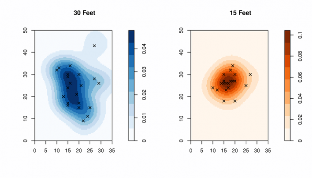
Figure: Density Comparison Pattern densities from the two experiments: 30 and 15 feet from target.
Load Data and Compute Density Maps:
### load some libraries
library(spatstat)
library(RColorBrewer)

## read in the data
t_30 <- read.csv('target_30.csv')
t_15 <- read.csv('target_15.csv')

## an initial plot
plot(t_30, xlim=c(0,35), ylim=c(0,50))
points(t_15, col='red')

## convert to spatstat objects
t_30.ppp <- ppp(t_30$x, t_30$y, xrange=c(0,35), yrange=c(0,50) )
t_15.ppp <- ppp(t_15$x, t_15$y, xrange=c(0,35), yrange=c(0,50) )

## check via plot
plot(t_30.ppp)
points(t_15.ppp, col='red')
Fit Point-Process Models:
## fit point-process model
t_30_fit <- ppm(t_30.ppp, ~polynom(x,y,3), Poisson())
t_15_fit <- ppm(t_15.ppp, ~polynom(x,y,3), Poisson())

## plot density comparisons between two ranges
par(mfcol=c(1,2))
plot( density(t_30.ppp), col=brewer.pal('Blues', n=9), main="30 Feet")
points(t_30.ppp, pch=4, cex=1)

plot( density(t_15.ppp), col=brewer.pal('Oranges', n=9), main="15 Feet")
points(t_15.ppp, pch=4, cex=1)


##
## plot a fit of the 30 foot pattern
##
par(mfcol=c(2,2))
plot( density(t_30.ppp), col=brewer.pal('Blues', n=9), main="30 Feet")
points(t_30.ppp, pch=4, cex=1)

plot(t_30_fit, col=brewer.pal('Blues', n=9), trend=TRUE, cif=FALSE, pause=FALSE, how="image")
plot(t_30_fit, trend=TRUE, cif=FALSE, pause=FALSE, how="contour")
plot(t_30_fit, colmap=brewer.pal('Blues', n=9), trend=TRUE, cif=FALSE, pause=FALSE, how="persp", theta=0, phi=45)


##
## plot a fit of the 15 foot pattern
##
par(mfcol=c(2,2))
plot( density(t_15.ppp), col=brewer.pal('Oranges', n=9), main="15 Feet")
points(t_15.ppp, pch=4, cex=1)

plot(t_15_fit, col=brewer.pal('Oranges', n=9), trend=TRUE, cif=FALSE, pause=FALSE, how="image")
plot(t_15_fit, trend=TRUE, cif=FALSE, pause=FALSE, how="contour")
plot(t_15_fit, colmap=brewer.pal('Oranges', n=9), trend=TRUE, cif=FALSE, pause=FALSE, how="persp", theta=0, phi=45)
Tidy-up: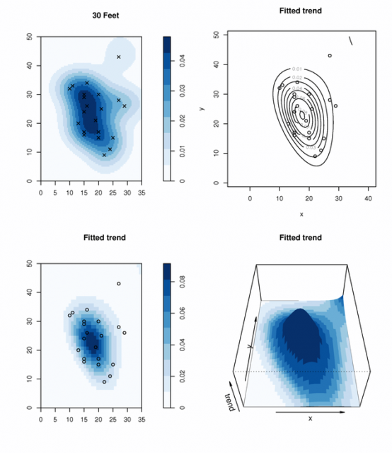
##
## convert to png:
for i in *.pdf ; do convert -density 300 +antialias $i `basename $i .pdf`.png ; done
for i in *.png ; do mogrify -reisize 25% $i ; done
Attachments:
Links:
Some Ideas on Interpolation of Categorical Data
Working with Spatial Data
Visual Interpretation of Principal Coordinates (of) Neighbor Matrices (PCNM)
