Convert Munsell colors to computer-friendly RGB triplets
The Munsell color system was designed as a series of discrete color chips which closely approximation to the color sensitivity of the human eye. The description of color via three variables tied to perceptible properties (hue, value, and chroma) under a standardized illuminant (sunlight on a clear day) makes the Munsell system a good choice for recording and interpreting soil color data. However, numerical analysis of colors encoded in the Munsell system is difficult because they are from a discrete set of color chips and referenced by values that include both letters and numbers. Rossel et. al. (2006) give a good background on various color space models and their relative usefulness in the realm of soil science. The conversion of Munsell soil colors to RGB triplets, suitable for displaying on a computer screen or printing, is made complicated by the numerous operations involved in converting between color spaces. Figure 1 shows all possible (both real and unreal) Munsell color chips in the L*U*V color space. Figure 2 shows some of the common soil color chips in the same color space. Figures 2 through 5 depict common soil colors in the RGB color space, visualized both in R and POVRAY. Example R code on the conversion is given below.
Munsell color data can be downloaded here.
Color conversion equations here.
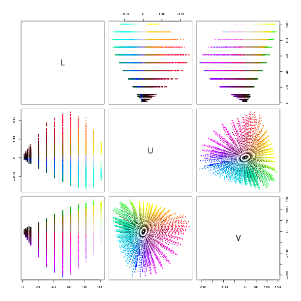 Figure 1: Munsell color chips. |
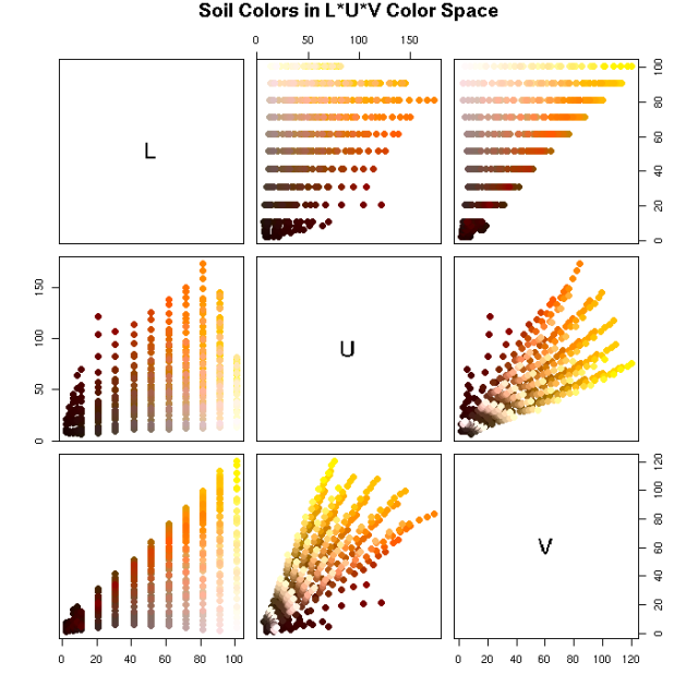 Figure 2: Common soil colors. |
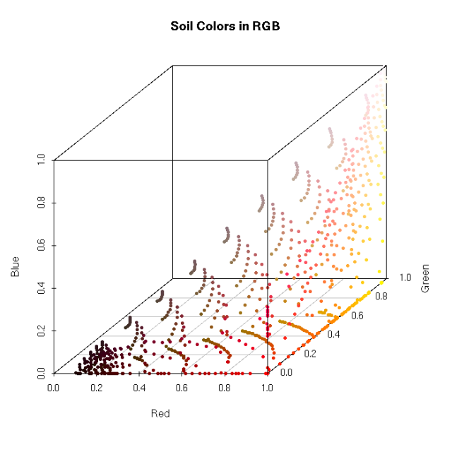 Figure 3: Commom soil colors in RGB |
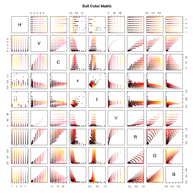 Figure 4: Soil colors in multiple color spaces |
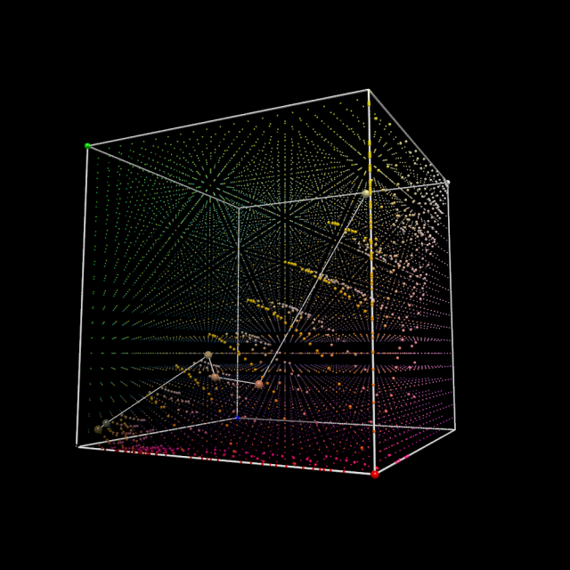 Figure 5: Soil profile colors. |
References:
- Rossel, R.A.V.; Minasny, B.; Roudier, P. & McBratney, A.B. Colour space models for soil science Geoderma, 2006, 133, 320-337.
Manual Conversion in R
Setup environment and load lookup table data
## load some libs
library(plotrix)
library(colorspace)

## munsell data comes with a lookup table in xyY colorspace
## url: http://www.cis.rit.edu/mcsl/online/munsell.php

## note:
## Munsell chroma, CIE x, y, and Y. The chromaticity coordinates were calculated using illuminant C and the CIE 1931 2 degree observer.
all <- read.table("munsell-all.dat", header=T)
Convert xyY to XYZ [Equation Reference]
## x and y are approx (0,1)
## Y is approx (0,100)

## need manually rescale Y to (0,1)
all$Y <- all$Y/100.0

## do the conversion
X <- (all$x * all$Y ) / all$y
Y <- all$Y
Z <- ( (1- all$x - all$y) * all$Y )  / all$y

## combine to form matrix for simple manipulation
mun_XYZ_C <- matrix(c(X,Y,Z), ncol=3)

## test for y == 0
## X,Y,Z should then be set to 0
mun_XYZ_C[which(all$y==0),] <- c(0,0,0)
Perform Chromatic Adaption Functions in the colorspace package, and sRGB profiles assume a D65 illuminant [Reference]
## conversion matrix, from reference above
## this has been revised as of Jan, 2008
M_adapt_C_to_D65 <- matrix(c(0.990448, -0.012371, -0.003564, -0.007168, 1.015594, 0.006770, -0.011615, -0.002928, 0.918157), ncol=3, byrow=TRUE)


## perform the chromatic adaption: convert from C -> D65 using Bradford method
mun_XYZ_D65 <- mun_XYZ_C %*% M_adapt_C_to_D65


## how different are the two?
summary( (mun_XYZ_D65 - mun_XYZ_C)  )
Convert XYZ (D65) to sRGB (D65), step 1 this assumes that XYZ is scaled to (0,1) [Reference Primaries for sRGB]
## first get the reference primaries transformation matrix from above
##
## sRGB profile transformation:
M_XYZ_to_sRGB_D65 <- matrix(c(3.24071, -0.969258, 0.0556352, -1.53726, 1.87599, -0.203996, -0.498571, 0.0415557, 1.05707), ncol=3, byrow=TRUE)

## apply the conversion matrix
mun_sRGB_D65 <- mun_XYZ_D65 %*% M_XYZ_to_sRGB_D65
Convert XYZ (D65) to sRGB (D65), step 2 (sRGB, gamma = 2.4) [Conversion Function to sRGB]
## define the transformation functions:
## these are applied on a conditional basis:
fun1 <- function(col_comp) { 1.055 * ( col_comp ^ ( 1 / 2.4 ) ) - 0.055 }
fun2 <- function(col_comp) { 12.92 * col_comp }

## the specific function is contingent on the absolute value of r,g,b components
R <- ifelse(mun_sRGB_D65[,1] > 0.0031308, fun1(mun_sRGB_D65[,1]), fun2(mun_sRGB_D65[,1]))
G <- ifelse(mun_sRGB_D65[,2] > 0.0031308, fun1(mun_sRGB_D65[,2]), fun2(mun_sRGB_D65[,2]))
B <- ifelse(mun_sRGB_D65[,3] > 0.0031308, fun1(mun_sRGB_D65[,3]), fun2(mun_sRGB_D65[,3]))


##clip values to range {0,1}
R_clip <- ifelse(R < 0, 0, R)
G_clip <- ifelse(G < 0, 0, G)
B_clip <- ifelse(B < 0, 0, B)

R_clip <- ifelse(R > 1, 1, R_clip)
G_clip <- ifelse(G > 1, 1, G_clip)
B_clip <- ifelse(B > 1, 1, B_clip)


## add these back to the original table:
all$R <- R_clip
all$G <- G_clip
all$B <- B_clip

## done with the conversion

## the manually converted data
plot( as(RGB(R_clip,G_clip,B_clip), 'LUV'), cex=0.5)
Attachment:
Software
- General Purpose Programming with Scripting Languages
- LaTeX Tips and Tricks
- PostGIS: Spatially enabled Relational Database Sytem
- PROJ: forward and reverse geographic projections
- GDAL and OGR: geodata conversion and re-projection tools
- R: advanced statistical package
- Access Data Stored in a Postgresql Database
- Additive Time Series Decomposition in R: Soil Moisture and Temperature Data
- Aggregating SSURGO Data in R
- Cluster Analysis 1: finding groups in a randomly generated 2-dimensional dataset
- Color Functions
- Comparison of Slope and Intercept Terms for Multi-Level Model
- Comparison of Slope and Intercept Terms for Multi-Level Model II: Using Contrasts
- Creating a Custom Panel Function (R - Lattice Graphics)
- Customized Scatterplot Ideas
- Estimating Missing Data with aregImpute() {R}
- Exploration of Multivariate Data
- Interactive 3D plots with the rgl package
- Making Soil Property vs. Depth Plots
- Numerical Integration/Differentiation in R: FTIR Spectra
- Plotting XRD (X-Ray Diffraction) Data
- Using lm() and predict() to apply a standard curve to Analytical Data
- Working with Spatial Data
- Comparison of PSA Results: Pipette vs. Laser Granulometer
- GRASS GIS: raster, vector, and imagery analysis
- Generic Mapping Tools: high quality map production

