
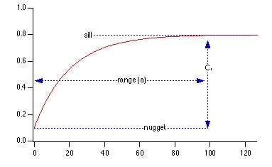
I have always had a hard time thinking about various parameters associated with random fields and empirical semi-variograms. The gstat package for R has an interesting interface for simulating random fields, based on a semi-variogram model. It is possible to quickly visualize the effect of altering semi-variogram parameters, by "seeding" the random number generator with the same value at each iteration. Of primary interest were visualization of principal axis of anisotropy, semi-variogram sill, and semi-variogram range. The code used to produce the images is included below. For more information on the R implementation of gstat, see the R-sig-GEO mailing list.
Setup
# load libraries
library(gstat)

# setup a grid
xy <- expand.grid(1:100, 1:100)
names(xy) <- c("x","y")
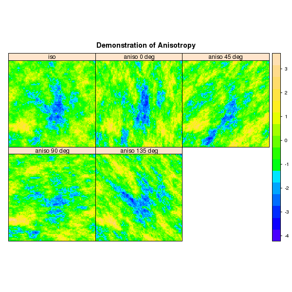
Demonstration of Anisotropy Direction
var.model <- vgm(psill=1, model="Exp", range=15)
set.seed(1)
sim <- predict(gstat(formula=z~1, locations= ~x+y, dummy=TRUE, beta=0, model=var.model, nmax=20), newdata = xy, nsim = 1)

var.model <- vgm(psill=1, model="Exp", range=15, anis=c(0, 0.5))
set.seed(1)
sim$sim2 <- predict(gstat(formula=z~1, locations= ~x+y, dummy=TRUE, beta=0, model=var.model, nmax=20), newdata=xy, nsim=1)$sim1

var.model <- vgm(psill=1, model="Exp", range=15, anis=c(45, 0.5))
set.seed(1)
sim$sim3 <- predict(gstat(formula=z~1, locations= ~x+y, dummy=TRUE, beta=0, model=var.model, nmax=20), newdata=xy, nsim=1)$sim1

var.model <- vgm(psill=1, model="Exp", range=15, anis=c(90, 0.5))
set.seed(1)
sim$sim4 <- predict(gstat(formula=z~1, locations= ~x+y, dummy=TRUE, beta=0, model=var.model, nmax=20), newdata=xy, nsim=1)$sim1

var.model <- vgm(psill=1, model="Exp", range=15, anis=c(135, 0.5))
set.seed(1)
sim$sim5 <- predict(gstat(formula=z~1, locations= ~x+y, dummy=TRUE, beta=0, model=var.model, nmax=20), newdata=xy, nsim=1)$sim1

# promote to SP class object
gridded(sim) = ~x+y

new.names <- c('iso', 'aniso 0 deg', 'aniso 45 deg', 'aniso 90 deg', 'aniso 135 deg')
p1 <- spplot(sim, names.attr=new.names, col.regions=topo.colors(100), as.table=TRUE, main="Demonstration of Anisotropy")
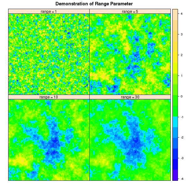
Figure: Demonstration of Range Parameter
Demonstrate Range Parameter
var.model <- vgm(psill=1, model="Exp", range=1)
set.seed(1)
sim <- predict(gstat(formula=z~1, locations= ~x+y, dummy=TRUE, beta=0, model=var.model, nmax=20), newdata = xy, nsim = 1)

var.model <- vgm(psill=1, model="Exp", range=5)
set.seed(1)
sim$sim2 <- predict(gstat(formula=z~1, locations= ~x+y, dummy=TRUE, beta=0, model=var.model, nmax=20), newdata=xy, nsim=1)$sim1

var.model <- vgm(psill=1, model="Exp", range=15)
set.seed(1)
sim$sim3 <- predict(gstat(formula=z~1, locations= ~x+y, dummy=TRUE, beta=0, model=var.model, nmax=20), newdata=xy, nsim=1)$sim1

var.model <- vgm(psill=1, model="Exp", range=30)
set.seed(1)
sim$sim4 <- predict(gstat(formula=z~1, locations= ~x+y, dummy=TRUE, beta=0, model=var.model, nmax=20), newdata=xy, nsim=1)$sim1

# promote to SP class object
gridded(sim) = ~x+y

new.names <- c('range = 1', 'range = 5', 'range = 10', 'range = 30')
p2 <- spplot(sim, names.attr=new.names, col.regions=topo.colors(100), as.table=TRUE, main="Demonstration of Range Parameter")
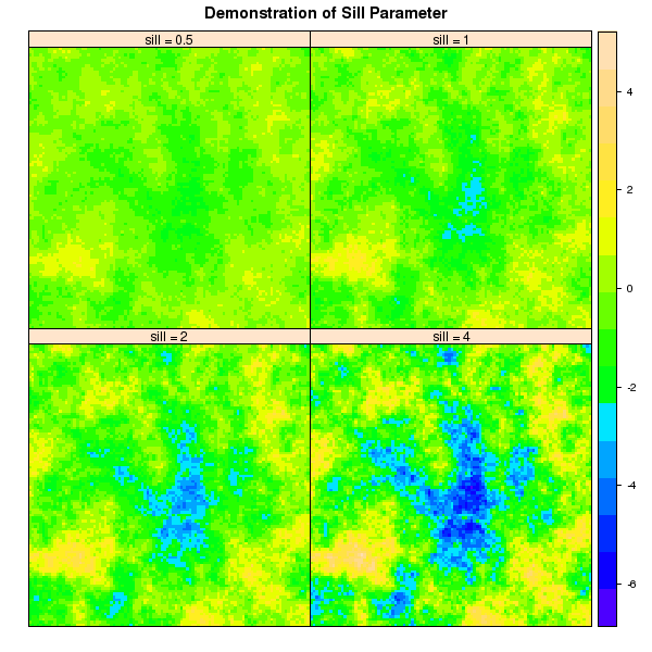
Demonstrate Sill Parameter
var.model <- vgm(psill=0.5, model="Exp", range=15)
set.seed(1)
sim <- predict(gstat(formula=z~1, locations= ~x+y, dummy=TRUE, beta=0, model=var.model, nmax=20), newdata = xy, nsim = 1)


var.model <- vgm(psill=1, model="Exp", range=15)
set.seed(1)
sim$sim2 <- predict(gstat(formula=z~1, locations= ~x+y, dummy=TRUE, beta=0, model=var.model, nmax=20), newdata=xy, nsim=1)$sim1

var.model <- vgm(psill=2, model="Exp", range=15)
set.seed(1)
sim$sim3 <- predict(gstat(formula=z~1, locations= ~x+y, dummy=TRUE, beta=0, model=var.model, nmax=20), newdata=xy, nsim=1)$sim1

var.model <- vgm(psill=4, model="Exp", range=15)
set.seed(1)
sim$sim4 <- predict(gstat(formula=z~1, locations= ~x+y, dummy=TRUE, beta=0, model=var.model, nmax=20), newdata=xy, nsim=1)$sim1

# promote to SP class object
gridded(sim) = ~x+y

new.names <- c('sill = 0.5', 'sill = 1', 'sill = 2', 'sill = 4')
p3 <- spplot(sim, names.attr=new.names, col.regions=topo.colors(100), as.table=TRUE, main="Demonstration of Sill Parameter")
Links:
Visual Interpretation of Principal Coordinates (of) Neighbor Matrices (PCNM)
Working with Spatial Data
Comparison of PSA Results: Pipette vs. Laser Granulometer
