
Premise
Wanted to make something akin to an interpolated surface for some spatially auto-correlated categorical data (presence/absence). I quickly generated some fake spatially auto-correlated data to work with using r.surf.fractal in GRASS. These data were converted into a binary map using an arbitrary threshold that looked about right-- splitting the data into something that looked 'spatially clumpy'.
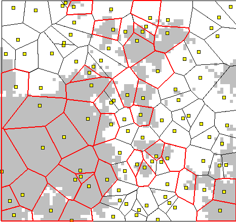
Fig. 1: Simulated auto-correlated, categorical variable, with sampling points and derived voronoi polygons.
I had used voronoi polygons in the past to display connectivity of categorical data recorded at points, even though sparsely sampled areas tend to be over emphasized. Figure 1 shows the fake spatially auto-correlated data (grey = presence /white = not present), sample points (yellow boxes), and voronoi polygons. The polygons with thicker, red boundaries represent the "voronoi interpolation" of the categorical feature.
Interpolation by RST
Wanting something a little more interesting, I tried interpolating the presence/absence data by via RST. Numerical interpolation of categorical data is usually not preferred as it creates a continuum between discreet classes-- i.e. values that do not have a sensible interpretation. Throwing that aside for the sake of making a neat map, a color scheme was selected to emphasize the categorical nature of the interpolated surface (Figure 2).
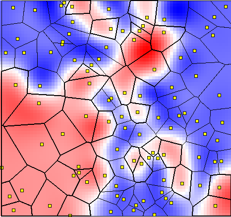
Fig. 2: RST interpolation of 0-1 continuum: red=1, blue=0.
Conditional Indicator Simulation
Finally, I gave conditional indicator simulation a try-- this required two steps: 1) fitting a model variogram, 2) simulation. This approach generates different output on each simulation, however, the output represents the original spatial pattern and variability. A more interesting map could be generated by running 1000 simulations and converting them into a single probability map.
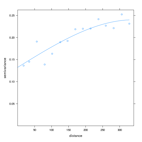
Indicator Variogram: Empirical semi-variogram for indicator=1, with spherical model fit.
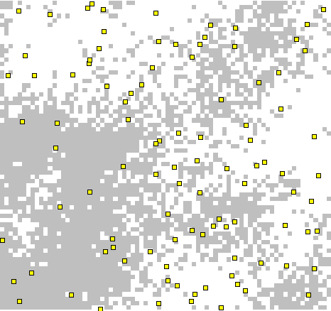
Categorical Interpolation 3: Single conditional indicator simulation.
Comparison
Code Snippets
Generate Some Data in GRASS
# set a reasonable resolution
g.region res=10 -ap

# simulate some spatially auto-correlated data
# and convert to categorical map
r.surf.fractal --o dimension=2.5 out=fractal
r.mapcalc "fractal.bin = if(fractal > 0, 1, 0)"
r.colors fractal.bin color=rules <<EOF
0 white
1 grey
EOF

v.random --o out=v n=100
v.db.addtable map=v
v.db.addcol map=v column="fractal double, class integer"
v.what.rast vect=v rast=fractal column=fractal
v.what.rast vect=v rast=fractal.bin column=class

# simplest approach
v.voronoi --o in=v out=v_vor

# try interpolation of classes...
v.surf.rst --o in=v zcol=class elev=v.interp
r.colors map=v.interp color=rules <<EOF
0% blue
0.5 white
100% red
EOF
Perform Indicator Simulation in R
# indicator simulation
library(spgrass6)
library(gstat)

# read vector
d <- readVECT6('v')

# convert class to factor
d@data <- transform(d@data, class=factor(class))

# inspect variogram of x$class == 1
plot(v <- variogram(I(class == 1) ~ 1, data = d))

# fit a spherical variogram with nugget
# not sure about the syntax
v.fit <- fit.variogram(v, vgm(psill=1, model='Sph', range='250', 1))

# png(file='indicator_variogram.png', width=400, height=400, bg='white')
plot(v, model=v.fit)
# dev.off()

# make a grid to predict onto
G <- gmeta6()
grd <- gmeta2grd()

# new grid
new_data <- SpatialGridDataFrame(grd, data=data.frame(k=rep(1,G$cols*G$rows)), proj4string=CRS(d@proj4string@projargs))


# conditional indicator simulation:
# need to study this syntax
# make more simulations for an estimated probabilitry
p <- krige(I(class == 1) ~ 1, d, new_data, v.fit, nsim=1, indicators=TRUE, nmax=40)

# write one back to GRASS
writeRAST6(p, 'indicator.sim', zcol='sim1')
Make Some Maps in GRASS
# fix colors of the simulated map
r.colors map=indicator.sim color=rules << EOF
0 white
1 grey
EOF


# simple maps
d.erase
d.rast v.interp
d.vect v icon=basic/box  size=7 fcol=yellow
d.vect v_vor type=area fcol=none where=class=0
d.vect v_vor type=area fcol=none width=2 where=class=1
d.out.file --o out=example1

d.erase
d.rast fractal.bin
d.vect v icon=basic/box  size=7 fcol=yellow
d.vect v_vor type=area fcol=none where=class=0
d.vect v_vor type=area fcol=none col=red width=2 where=class=1
d.out.file --o out=example2

d.erase
d.vect v_vor type=area fcol=white where=class=0
d.vect v_vor type=area fcol=grey where=class=1
d.vect v icon=basic/box  size=7 fcol=yellow
d.out.file --o out=example3

d.erase
d.rast indicator.sim
d.vect v icon=basic/box size=7 fcol=yellow
d.out.file --o out=example4
Links:
Simple Map Creation
Working with Spatial Data
Target Practice and Spatial Point Process Models
