
Comparison of PSA Results: Pipette vs. Laser Granulometer
Soil texture data was collected via pipette and laser granulometer, each horizon from three pedons. This example illustrates a simple approach to comparing the two methods with both standard XY-style scatter plot and on a soil textural triangle. This example uses code in the plotrix package for R, but you could also use this pythonapproach.
The data referenced in these examples are attached at the bottom of this page. The code boxes below represent what a user would type into the R console. Lines prefixed with a '#' are interpreted by R as a comment, and thus ignored. Further visualization examples, using a larger dataset, can be accessed by clicking on the link at the bottom of this page. The goals of this example are:
- import data into R
- plot data
- perform a simple linear regression
- plot sand, silt, clay data on a textural triangle
Example commands can be directly pasted into the R console, or typed by hand. I would recommend copyinf a single line of example code at a time into the R console, then press the ENTER key. In this way the results of each command will be visible. Remember that the str() function will give you information about an object. Note that in order to load the sample data, you will need to set your working directory in R to the same folder in which you downloaded the sample data. For example: if you downloaded the sample data to your Desktop, you would set your working directory with:
- on a mac: setwd('~/Desktop')
- on windows: setwd('C:\path_to_your_desktop') where 'path_to_your_desktop' is the path to the desktop folder
Optionally, you can use the file.choose() command to bring up a standard file selection box. The result of this function can then be pasted into the read.table('....') function, replacing the '...' with the data returned from file.choose()
 Sample Plot: Pipette vs. Granulometer |
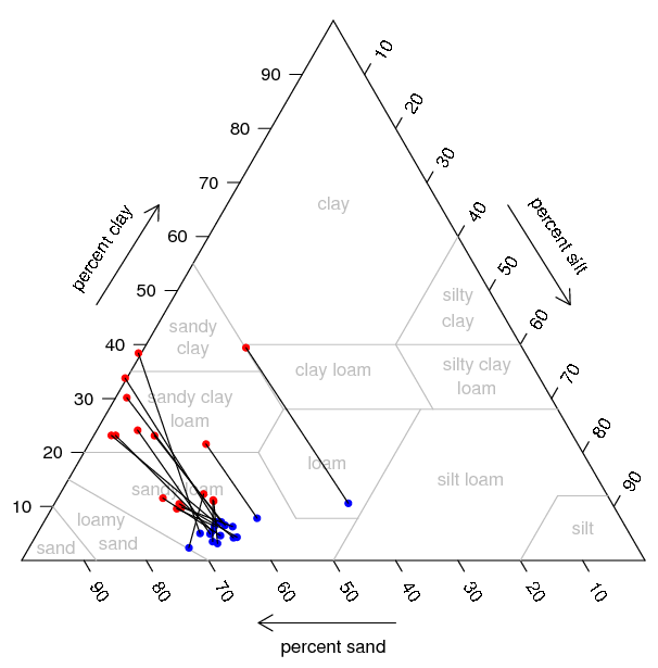 Sample Plot: Soil Textural Triangle: pipette values are in red, granulometer values are in blue. Line segments connect corresponding observations. |
Load Required Packages and Input Data
# the package 'plotrix' can be installed with:
# install.packages('plotrix', repos='http://cran.r-project.org', dependencies=TRUE)
# note 1: you can accomplish this through the R-GUI in windows / mac os
# note 2: on UNIX-like systems you will need to start R as superuser to install packages
# load required package
require(plotrix)

#read in text data: note that they are TAB-DELIMITED: <b>sep='\t'</b>
p <- read.table('psa-pipette.txt', header=T, sep="\t")

#note that the granulometer data is whitesdpace delimeted: i.e. no 'sep=' argument
g <- read.table('gran-psa.txt', header=T)
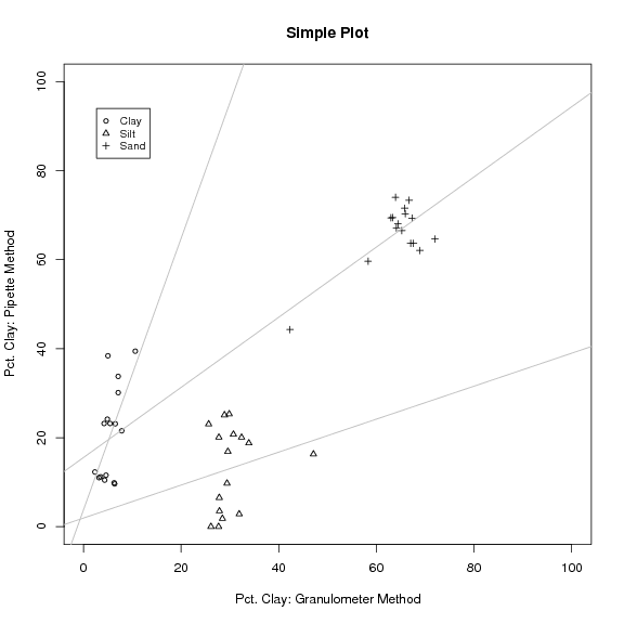
Initial Comparison of Clay Values See Figure 1
#do some initial comparisons:
plot(p$clay ~ g$clay)

#re-plot with custom settings:
# annotated axis, 0-100% range, plot symbols scaled by 0.8
plot(p$clay ~ g$clay, ylab="Pct. Clay: Pipette Method", xlab="Pct. Clay: Granulometer Method", main="Simple Plot", xlim=c(0,100), ylim=c(0,100), cex=0.8)

#add silt fraction to the SAME plot:
points(p$silt ~ g$silt,  cex=0.8, pch=2)
# add sand fraction to the SAME plot:
points(p$sand ~ g$sand,  cex=0.8, pch=3)

#add a legend:
legend(x=2.7, y=94, legend=c('Clay','Silt','Sand'), pch=1:3, cex=0.8)

#simple linear modeling: add trend lines
abline(lm(p$clay ~ g$clay), col="gray")
abline(lm(p$silt ~ g$silt), col="gray")
abline(lm(p$sand ~ g$sand), col="gray")
Simple Linear Model
#create a formular object
f <- p$clay ~ g$clay
#create a model object
m <- lm( f )
#return the details on the new model:
summary( m )

#the following is the output:

Call:
lm(formula = p$clay ~ g$clay)

Residuals:
     Min       1Q   Median       3Q      Max
-13.6120  -6.1412   0.4438   4.8047  19.3997

Coefficients:
            Estimate Std. Error t value Pr(>|t|)
(Intercept)    3.761      6.477   0.581   0.5707
g$clay         3.052      1.093   2.793   0.0144 *
---
Signif. codes:  0 ‘***’ 0.001 ‘**’ 0.01 ‘*’ 0.05 ‘.’ 0.1 ‘ ’ 1

Residual standard error: 8.664 on 14 degrees of freedom
Multiple R-Squared: 0.3577,     Adjusted R-squared: 0.3119
F-statistic: 7.798 on 1 and 14 DF,  p-value: 0.01439
Sample soil texture data plotted on the texture triangle See Figure 2
#subset sand, silt, clay information for texture triangle plot:
p.ssc <- data.frame(sand=p$sand,silt=p$silt,clay=p$clay)
g.ssc <- data.frame(sand=g$sand,silt=g$silt,clay=g$clay)

#plot a texture triangle from the pipette data
p.tri <- soil.texture(p.ssc,show.lines=T, show.names=T, tick.labels=seq(10,90,10), col.symbol='red', pch=16, cex=0.8, main="Soil Texture Triangle")
#add points from the granulometer data
g.tri  <- triax.points(g.ssc, col.symbol='blue', pch=16, cex=0.8)

#plot segments connecting (also see 'arrows' function)
segments(p.tri$x, p.tri$y, g.tri$x, g.tri$y, col='black', lty=1)
