
Point-process modelling with the sp and spatstat packages
Some simple examples of importing spatial data from text files, converting between R datatype, creation of a point process model and evaluating the model. Input data sources are: soil pit locations with mollic and argillic diagnostic horizons (mollic-pedons.txt and argillic-pedons.txt), and a simplified outline of Pinnacles National Monument (pinn.txt). The outline polygon is used to define a window in which all operations are conducted.
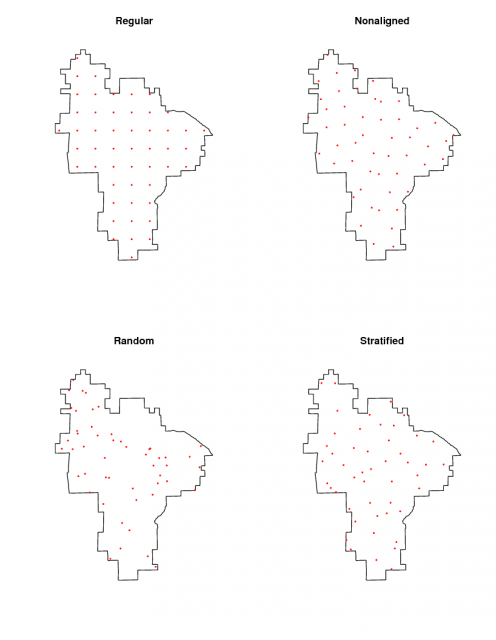
The 'sp' package for R contains the function spsample(), can be used to create a sampling plan for a given region of interest: i.e. the creation of n points within that region based on several algorithms. This example illustrates the creation of 50 sampling points within Pinnacles, according to the following criteria: regular (points are located on a regular grid), nonaligned (points are located on a non-aligned grid-like pattern), random (points are located at random), stratified (collectively exhaustive, see details here).
The 'spatstat' package for R contains several functions for creating point-process models: models describing the distribution of point events: i.e. the distribution of tree species within a forest. If covariate data is present (i.e. gridded precipitation, soil moisture, aspect, etc.) these covariates can be incorporated into the point-process model. Without covariate data, the model is based on an spatial distribution estimator function. Note that the development of such models is complicated by factors such as edge-effects, degree of stochasticity, spatial connectivity, and stationarity. These are rather contrived examples, so please remember to read up on any functions you plan to use for your own research. An excellent tutorial on Analyzing spatial point patterns in R was recently published.
Helpful links
Spatstat Quick Reference
Print Version with Links
 Four sampling designs |
 Spatial density of each pedon type |
 Spatial density of the four sampling designs |
 Example point-process model of mollic soils |
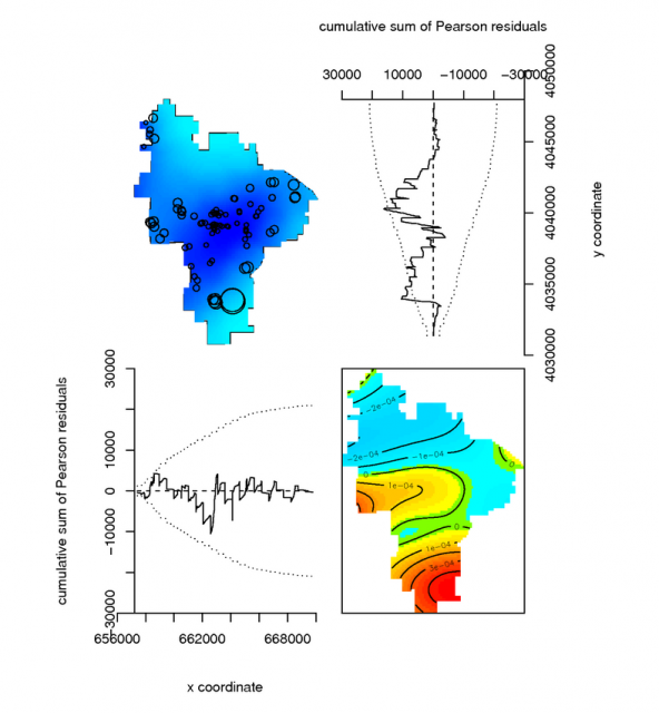 Diagnostics of a simple point-process model |
Note: This code should be updated to use the slot() function instead of the '@' syntax for accessing slots!
Load required packages and input data (see attached files at bottom of this page)
# load required packages
library(sp)
library(spatstat)

# read in pinnacles boundary polygon: x,y coordinates
# use the GRASS vector, as it should be topologically correct
# v.out.ascii format=standard in=pinn_bnd > pinn.txt ... edit out extra crud
pinn <- read.table('pinn.txt')

# read in mollic and argillic pedons
# see ogrinfo hack
m <- read.table('mollic-pedons.txt', col.names=c('x','y'))
a <- read.table('argillic-pedons.txt', col.names=c('x','y'))

# add a flag for the type of pedon
m$type <- factor('M')
a$type <- factor('A')

#combine into a single dataframe
pedons <- rbind.data.frame(a,m)
Using the functions from the 'sp' package create a polygon object from the pinn.txt coordinates
# create a spatial polygon class object
pinn.poly <- SpatialPolygons(list(Polygons(list(Polygon( pinn )), "x")))

# inspect this new object with str()
# total area of all polygons
pinn.poly@polygons[[1]]@area

# coordinates of first polygon: this is rough syntax!
pinn.poly@polygons[[1]]@Polygons[[1]]@coords
Generate a sampling plan for 50 sites using regular grid, non-aligned grid, random, and random stratified approaches
# generate random points within the pinnacled boundary
p.regular <- spsample(pinn.poly, n = 50, "regular")
p.nalign <- spsample(pinn.poly, n = 50, "nonaligned")
p.random <- spsample(pinn.poly, n = 50, "random")
p.stratified <- spsample(pinn.poly, n = 50, "stratified")

# setup plot environment
par(mfrow=c(2,2))

# each of the sampling designs
plot(pinn.poly)
title("Regular")
points(p.regular, pch=16, col='red', cex=0.3)

plot(pinn.poly)
title("Nonaligned")
points(p.nalign, pch=16, col='red', cex=0.3)

plot(pinn.poly)
title("Random")
points(p.random, pch=16, col='red', cex=0.3)

plot(pinn.poly)
title("Stratified")
points(p.stratified, pch=16, col='red', cex=0.3)
Convert 'sp' class objects to 'spatstat' analogues note the use of 'slots'
 # pinn boundary:
# extract coordinates: and get a length - 1 value
p.temp <- pinn.poly@polygons[[1]]@Polygons[[1]]@coords
n <- length(p.temp[,1]) - 1

# create two vectors: x and y
# these will contain the reversed vertices, minus the last point
# in order to adhere to the spatstat specs: no repeating points, in counter-clockwise order
x <- rev(p.temp[,1][1:n])
y <- rev(p.temp[,2][1:n])

# make a list of coordinates: note that we are removing the last vertex
p.list <- list(x=x,y=y)

# make a spatstat window object from the polygon vertices
W <- owin(poly=p.list)

# pedons with their 'marks' i.e. pedon type, and the pinn boundary as the 'window'
pedons.ppp <- ppp(pedons$x, pedons$y, xrange=c(min(pedons$x), max(pedons$x)), yrange=c(min(pedons$y), max(pedons$y)) , window=W, marks=pedons$type)
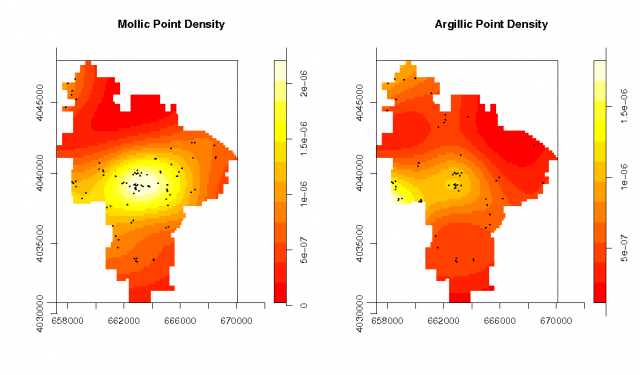
Plot and summarize the new combined set of pedon data
# plot and summarize the pedons data:
# note the method used to subset the two 'marks'
par(mfrow=c(1,2))
plot(density.ppp(pedons.ppp[pedons.ppp$marks == 'M']), main="Mollic Point Density")
points(pedons.ppp[pedons.ppp$marks == 'M'], cex=0.2, pch=16)

plot(density.ppp(pedons.ppp[pedons.ppp$marks == 'A']), main="Argillic Point Density")
points(pedons.ppp[pedons.ppp$marks == 'A'], cex=0.2, pch=16)

summary(pedons.ppp)

Marked planar point pattern: 151 points
Average intensity 1.38e-06 points per unit area
Marks:
frequency proportion intensity
A 62 0.411 5.67e-07
M 89 0.589 8.14e-07

Window: polygonal boundary
single connected closed polygon with 309 vertices
enclosing rectangle: [ 657228.3125 , 670093.8125 ] x [ 4030772.75 , 4047986.25 ]
Window area = 109337135.585938
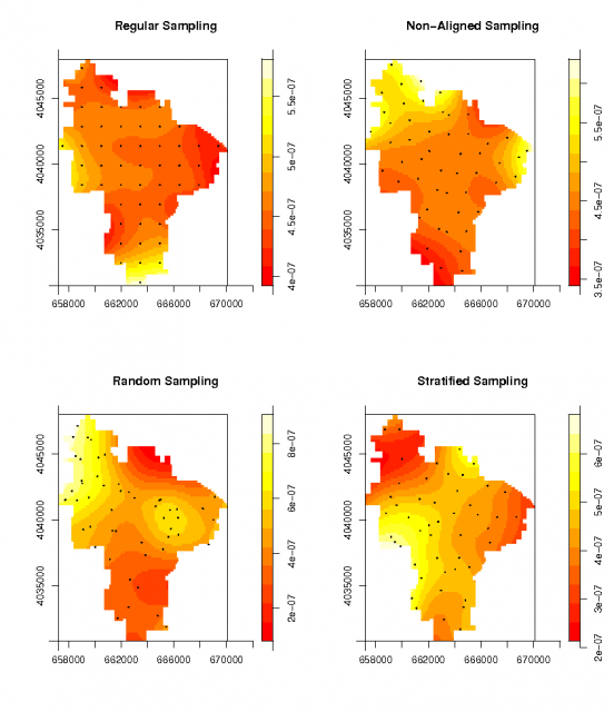
Convert the sampling design points (from above) to 'spatstat' objects and plot their density
# convert the random datasets: using the same window:
ppp.regular <- ppp(p.regular@coords[,1], p.regular@coords[,2], window=W)
ppp.nalign <- ppp(p.nalign@coords[,1], p.nalign@coords[,2], window=W)
ppp.random <- ppp(p.random@coords[,1], p.random@coords[,2], window=W)
ppp.stratified <- ppp(p.stratified@coords[,1], p.stratified@coords[,2], window=W)

# visually check density of random points:
par(mfrow=c(2,2))
plot(density.ppp(ppp.regular), main="Regular Sampling")
points(ppp.regular, pch=16, cex=0.2)

plot(density.ppp(ppp.nalign), main="Non-Aligned Sampling")
points(ppp.nalign, pch=16, cex=0.2)

plot(density.ppp(ppp.random), main="Random Sampling")
points(ppp.random, pch=16, cex=0.2)

plot(density.ppp(ppp.stratified), main="Stratified Sampling")
points(ppp.stratified, pch=16, cex=0.2)
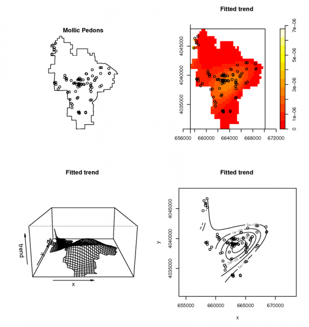
Simple, and probably flawed attempt to use a point-process model for the pedon data Third order polynomial model for the distribution of pedons with a mollic epipedon. See manula page for ppm() for detailed examples.
# model the spatial occurance of Mollic epipedons with a 3rd-order polynomial, using the Poisson Process Theory
fit <- ppm( unmark(pedons.ppp[pedons.ppp$marks == 'M']), ~polynom(x,y,3), Poisson())

# view the fitted model
par(mfcol=c(2,2))
plot(unmark(pedons.ppp[pedons.ppp$marks == 'M']), main="Mollic Pedons")
plot(fit)

# plot some diagnostics on the fitted model: Pearson residuals (see references)
diagnose.ppm(fit, type="pearson")


#another example using a buil-in dataset: the Lansing Forest
# fit nonstationary marked Poisson process
# with different log-cubic trend for each species
data(lansing)
fit <- ppm(lansing, ~ marks * polynom(x,y,3), Poisson())
plot(fit)
Point-process model diagnostic references from the spatstat manual
Baddeley, A., Turner, R., Moller, J. and Hazelton, M. (2005) Residual analysis for spatial point processes. Journal of the Royal Statistical Society, Series B 67, 617–666.
Stoyan, D. and Grabarnik, P. (1991) Second-order characteristics for stochastic structures connected with Gibbs point processes. Mathematische Nachrichten, 151:95–100.
