
Interactive 3D plots with the rgl package
Overview
Sample application of the RGL package. This package allows for the creation of interactive, 3D figures, complete with lighting and material effects. Try demo(rgl)for an idea of what is possible.
A random number generator sphere (RNG sphere) was created based on the suggestions in Keys to Infinity by Clifford A. Pickover, pp. 237-239. The RNG sphere can be used to test the robustness of a random number generator. Three random number generators were tested: runif() from R, rand from Excel, and a logistic-derived psudo-random number generator. The location (x,y,z) and color of the spheres are based on the sequence of random numbers (Pickover, 1995). An ideal RNG shpere should have no discernable patterns. Note that the logistic-derived random numbers show distinct correlation in the RNG sphere. Excel random number list, and source code (R) are attached at the botom of the page.
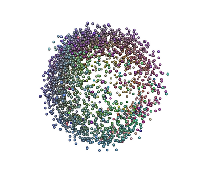
RGL sample application: 3d interactive interface to a random number generator sphere. Random numbers from runif() function in R.
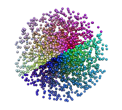
RGL sample application 2: Excel random number visualization: 3d interactive interface to a random number generator sphere. Random numbers from rand() function in MS Excel.
RGL sample application 2: Random numbers from the logistic function: 3d interactive interface to a random number generator sphere. Random numbers from the logistic function (see notes), implemented in R.
Random Number Generator (RNG) Sphere Function Definition
 # simple function for
rng_sphere <- function(d, type='rgl')
{

n <- length(d)
nn <- n - 3

# init our x,y,z coordinate arrays
x <- array(dim=nn)
y <- array(dim=nn)
z <- array(dim=nn)

# init red,green,blue color component arrays
cr <- array(dim=nn)
cg <- array(dim=nn)
cb <- array(dim=nn)


# convert lagged random numbers from d into spherical coordinates
# then convert to cartesian x,y,z coordinates for simple display
for (i in 1:nn)
{
theta <- 2*pi*d[i]
phi <- pi*d[i+1]
r <- sqrt(d[i+2])

x[i] <- r * sin(theta) * cos(phi)
y[i] <- r * sin(theta) * sin(phi)
z[i] <- r * cos(theta)

# give each location a color based on some rules
cr[i] <- d[i] / max(d)
cg[i] <- d[i+1] / max(d)
cb[i] <- d[i+2] / max(d)

} # end function


if( type == 'rgl')
{
# setup rgl environment:
zscale <- 1

# clear scene:
clear3d("all")

# setup env:
bg3d(color="white")
light3d()

# draw shperes in an rgl window
spheres3d(x, y, z, radius=0.025, color=rgb(cr,cg,cb))
}

if(type == '2d')
{
# optional scatterplot in 2D
scatterplot3d(x,y,z, pch=16, cex.symbols=0.25, color=rgb(cr,cg,cb), axis=FALSE )
}


# optionally return results
# list(x=x, y=y, z=z, red=cr, green=cg, blue=cb)

}
Sample
# load required packages
require(scatterplot3d)
require(rgl)

# random number with runif():
d <- runif(2500)

# plot rng sphere with rgl:
rng_sphere(d, type='rgl')

# save results of the rgl window
rgl.snapshot('testing.png')

# plot rng sphere with scatterplot3d:
rng_sphere(d, type='2d')

# save results
dev.copy2eps()

# 2500 excel random numbers
# =rand()
dd <- as.vector(unlist(read.csv('excel_rand.csv')))
rng_sphere(dd, type='rgl')
rgl.snapshot('testing-excel.png')


# 1000 random numbers from the logistic function:

# init an array
ddd <- array(dim=1000)

# seed
ddd[1] <- 0.38273487234

# compute for the next 999 iterations
for (i in 1:999) { ddd[i+1] <- 4 * 1 * ddd[i] * (1 - ddd[i]) }
