Comparison of Slope and Intercept Terms for Multi-Level Model
Jan 29, 2009 metroadminPremise
When the relationship between two variable is (potentially) dependent on a third, categorical variable ANCOVA (analysis of covariance), or some variant, is commonly used. There are several approaches to testing for differences in slope/intercepts (in the case of a simple linear model) between levels of the stratifying variable. In R the following formula notation is usually used to test for interaction between levels of a factor (f) and the relationship between two continuous variables x and y: y ~ x * f. A simple graphical exploration of this type of model can be done through examination of confidence intervals computed for slope and intercept terms, for each level of our grouping factor (f). An example of a fictitious dataset is presented below. Note that this a rough approximation for testing differences in slope/intercept within a multi-level model. A more robust approach would take into account that we are trying to make several pair-wise comparisons, i.e. something akin to Tukey's HSD. Something like this can be done with the multcomp package. For any real data set you should always consult a real statistician.

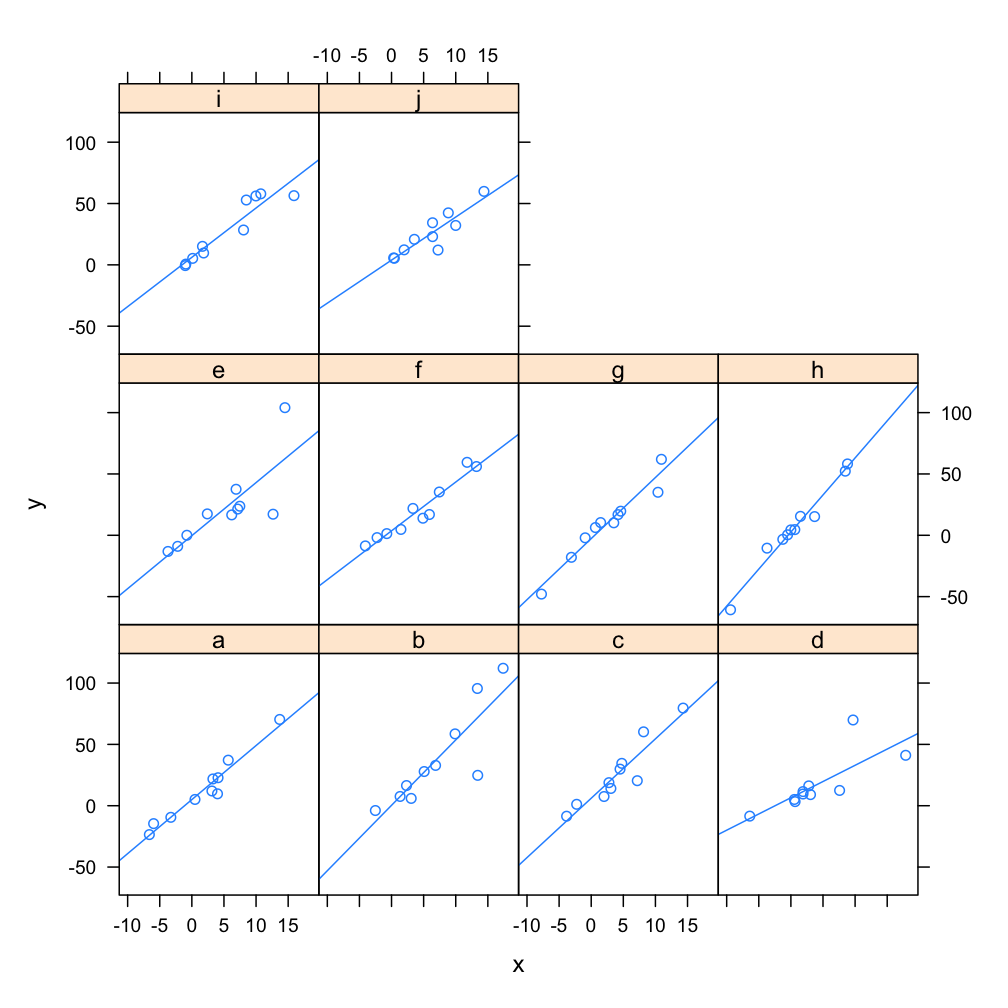
Example Multi-Level Model: each panel represents a model fit to y ~ x, for group f
Example Multi-Level Data
# need this for xyplot()
library(lattice)

# make some fake data:
x <- rnorm(100, mean=3, sd=6)
y <- x * runif(100, min=1, max=7) + runif(100, min=1.8, max=5)
d <- data.frame(x, y, f=rep(letters[1:10], each=10))

# check it out
xyplot(y ~ x | f, data=d, type=c('p','r'))
Implementation

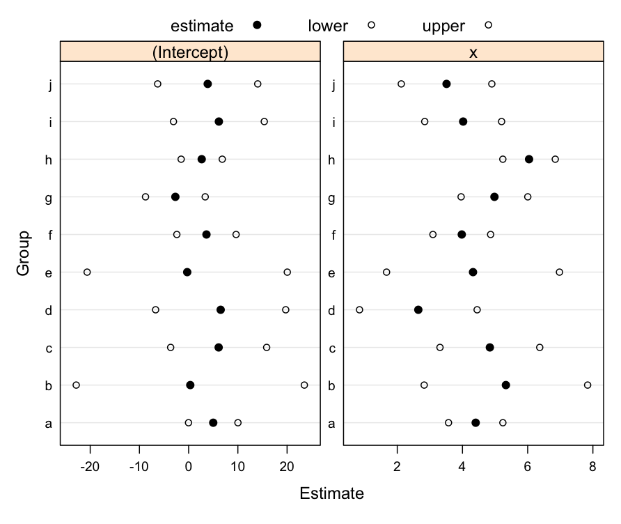
Example Multi-Level Model: Confidence Intervals: parameter estimates along with 95% confidence interval, within each level of our grouping factor (f).
Automated Plotting of Parameter Confidence Intervals
# split by factor
d.l <- split(d, d$f)
# fit model for each level of factor
fits <- lapply(d.l, function(d_i) {lm(y ~ x, data=d_i)})

# extract coefs
est <- lapply(fits, coef)

# compute confints
ci <- lapply(fits, confint)

ci.mat <- do.call('rbind', ci)
est.mat <- do.call('rbind', est)
ci.df <- data.frame(f=rep(colnames(sapply(ci, '[')), each=2))
ci.df$lower <- ci.mat[,1]
ci.df$upper <- ci.mat[,2]

# re-attach estimate label
ci.df$which <- row.names(ci.mat)

# add dummy column for estimate
ci.df$estimate <- NA

# make a data frame for the estimates
est.df <- data.frame(which=rep(colnames(est.mat), each=nrow(est.mat)))
est.df$estimate <- as.vector(c(est.mat[,1], est.mat[,2]))
est.df$f <- rep(row.names(est.mat), 2)

# add dummy columns for upper and lower conf ints
est.df$upper <- NA
est.df$lower <- NA

# combine estimate with confints
combined <- rbind(est.df, ci.df)

# combined plot of estimate +/- confint
dotplot(f ~ estimate + lower + upper | which, data=combined, scales=list(relation='free'), xlab="Estimate", ylab="Group", auto.key=list(columns=3),
par.settings=list(superpose.symbol=list(col=c(1), pch=c(16,1,1), cex=c(1,0.75,0.75))))
Formal Evaluation with lm()
The first two lines in the output below are testing the hypothesis that the slope and intercept term for level 'a' are not different than 0. Subsequent hypothesis tests are relative to the first 'level' in the dataset. In this case we are testing the hypothesis that intercept and slope terms for levels 'b' through 'j' are not different than the corresponding terms for level 'a'. From the output below we can see that none of the intercept terms (levels 'b' through 'j') are different than for 'a', and that the slope term for level 'd' is only marginally "different" (p=0.0625) than the slope term for 'a'.
Testing Model Terms
            Estimate Std. Error t value Pr(>|t|)
(Intercept)  4.99570    4.10909   1.216   0.2276
x            4.40546    0.68230   6.457 7.68e-09 ***
fb          -4.66364    7.28233  -0.640   0.5237
fc           1.10173    6.52890   0.169   0.8664
fd           1.51033    6.20212   0.244   0.8082
fe          -5.28549    6.62921  -0.797   0.4276
ff          -1.37673    6.39280  -0.215   0.8300
fg          -7.69480    5.93011  -1.298   0.1982
fh          -2.34349    5.70703  -0.411   0.6824
fi           1.14558    6.84805   0.167   0.8676
fj          -1.12319    7.87523  -0.143   0.8869
x:fb         0.92661    0.94257   0.983   0.3285
x:fc         0.43454    1.04819   0.415   0.6796
x:fd        -1.75956    0.93137  -1.889   0.0625 .
x:fe        -0.08193    0.96216  -0.085   0.9323
x:ff        -0.42669    0.99172  -0.430   0.6682
x:fg         0.57531    0.99279   0.579   0.5639
x:fh         1.63650    1.02319   1.599   0.1137
x:fi        -0.38424    0.97753  -0.393   0.6953
x:fj        -0.89373    1.14337  -0.782   0.4367
Links:
Using ColorBrewer to assist with thematic map color selection
R: advanced statistical package
Comparison of Slope and Intercept Terms for Multi-Level Model II: Using Contrasts
Software
- General Purpose Programming with Scripting Languages
- LaTeX Tips and Tricks
- PostGIS: Spatially enabled Relational Database Sytem
- PROJ: forward and reverse geographic projections
- GDAL and OGR: geodata conversion and re-projection tools
- R: advanced statistical package
- Access Data Stored in a Postgresql Database
- Additive Time Series Decomposition in R: Soil Moisture and Temperature Data
- Aggregating SSURGO Data in R
- Cluster Analysis 1: finding groups in a randomly generated 2-dimensional dataset
- Color Functions
- Comparison of Slope and Intercept Terms for Multi-Level Model
- Comparison of Slope and Intercept Terms for Multi-Level Model II: Using Contrasts
- Creating a Custom Panel Function (R - Lattice Graphics)
- Customized Scatterplot Ideas
- Estimating Missing Data with aregImpute() {R}
- Exploration of Multivariate Data
- Interactive 3D plots with the rgl package
- Making Soil Property vs. Depth Plots
- Numerical Integration/Differentiation in R: FTIR Spectra
- Plotting XRD (X-Ray Diffraction) Data
- Using lm() and predict() to apply a standard curve to Analytical Data
- Working with Spatial Data
- Comparison of PSA Results: Pipette vs. Laser Granulometer
- GRASS GIS: raster, vector, and imagery analysis
- Generic Mapping Tools: high quality map production

