
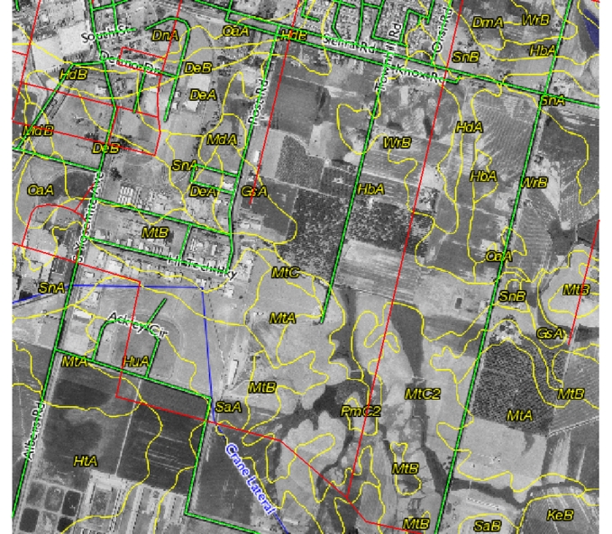
Example of bad Tiger data in Stanislaus County: Red lines are the original road network, green lines are the corrected road network.
The Problem
The US Census does a nice job of collecting all sorts of geographic and demographic information every 10 years. This data is available free of charge in the rather complex and soon to be replaced TIGER/LINE format. While this data covers the entire US down to the local road level, there are numerous errors and even extreme cases of coordinate-shift. Here is an example from Stanislaus County, California. The original TIGER data (red lines) are offset several hundred meters from the imagery. While it is not clear what may have caused the problem, it can be fixed without much effort using an affine transformation. We do not have the transformation matrix, however it can be 'fit' to a set of control points by several methods. The general form of the affine transform can be conveniently represented in homogeneous coordinates as:
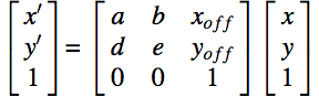
Affine Matrix Form in homogeneous coordinates:New coordinates on the left-hand side, old coordinates on the right-hand side. The transformation matrix is the 3x3 matrix in the center.
The Solution
- transform using GRASS and a set of control points with v.transform. This is the natural choice if the data is already in GRASS.
- Using the same control points, compute the transformation matrix in R, then apply in PostGIS with the Affine() function. This is the ideal approach for our scenario. Note that the format of the 'fitted' transformation matrix returned by R is in a slightly different format:
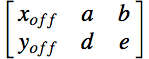 Transformation Matrix from R
We first need a set of control points, good and bad coordinates. This can be accomplished in several ways, we used the d.where command in GRASS:
# load road subset:
v.in.ogr dsn=PG:'dbname=tiger2005se user=xxx password=xxx host=xxx' layer=stan_roads out=s
#
# pick up some control points: note that they will be interleaved with this approach
# odd line numbers are "bad" coordinates
# even line numbers are "good" coordinates
d.where > stan.c_points
#
# we can separate the "bad" and "good" points in R...
Computing the transformation matrix can be done with a simple regression between 'good' and 'bad' coordinates in R. Note that this approach was suggested by Prof. Brian Ripley on the R-help mailing list.
Compute the Affine Transformation Matrix in R
## read in control points
## the good and bad points are interleaved
## odd numbers are 'bad' points
## s <- read.table('stan.c_points')

## s.bad <- s[seq(from=1, to=nrow(s), by=2), ]
## s.good <- s[seq(from=2, to=nrow(s), by=2), ]
##
## make a composite dataframe
## x,y = bad data
## nx,ny = good data
## c <- data.frame(x=s.bad$V1, y=s.bad$V2, nx=s.good$V1, ny=s.good$V2)
##
## save a local copy in the format that v.transform uses
## write.table(c, file='grass_control_pts.txt', row.names=F, col.names=F)
##

## from now on just use the simplified format:
c <- read.table('grass_control_pts.txt')
names(c) <- c('x','y','nx','ny')


## compute transformation matrix, and check model fit:
l <- lm(cbind(nx,ny) ~ x + y, data=c)
##
## see at bottom of page -->
summary(l)


## convert to affine transform matrix to the form needed by PostGIS:
## transpose the regression coefficient matrix:
t(coef(l))
 (Intercept)           x          y
nx    5017.082  1.00231639 0.00918962
ny  -28138.395 -0.01352029 0.99740077


## check graphically:
x <- seq(-2080000, -2040000, by=1000)
y <- seq(-20000, 5000, by=2000)
d <- expand.grid(x=x, y=y)
p <- predict(l, d)


par(mfcol=c(1,2), pty='s')
plot(y ~ x, data=c, main='Control Points', cex=.4, pch=16)
points(ny ~ nx, data=c, col='red', cex=.4, pch=16)
## arrows(c$x, c$y, c$nx, c$ny, len=0.05, col='gray')


plot(d, cex=0.2, main='Shifted Grid')
## arrows(d$x, d$y, p[,1], p[,2], len=0.05, col='gray')
points(p, col='red', cex=.2)


## sample transformation
print(predict(l, data.frame(x=-2078417.35893968, y=-14810.57043808)), digits=10)
            nx           ny
 -2078350.804 -14809.67334
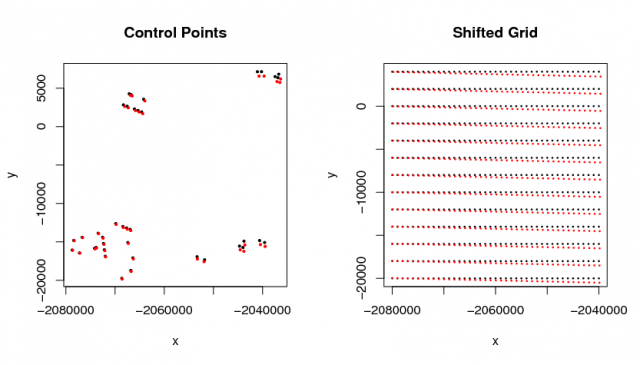
Establishing the transformation based on control points: Red points represent where the coordinates should be. Black points are the original and incorect coordinates.
Check Affine Transform Results in PostGIS
-- matrix format:

-- R:
-- | xoff a b |
-- | yoff d e |

-- postgis wants:
-- ST_Affine(geom, a, b, d, e, xoff, yoff)

-- as a query:
SELECT asText(
ST_Affine(
'POINT(-2078417.35893968 -14810.57043808)',
1.00231639, 0.00918962, -0.01352029, 0.99740077, 5017.082, -28138.395
)
) ;

                   astext
--------------------------------------------
 POINT(-2078350.80564006 -14809.6639251817)

-- This is the same as what R says!
Perform Affine Transformation in PostGIS
--
-- Step 1. Alter the geometry of the bad data in-place
-- note that we have a backup in 'stan_roads'
--
UPDATE roads SET wkb_geometry =  ST_Affine(wkb_geometry, 1.00231639, 0.00918962, -0.01352029, 0.99740077, 5017.082, -28138.395 ) WHERE module = 'TGR06099' ;
Regression Diagnostics
Response nx :

Call:
lm(formula = nx ~ x + y, data = d)

Residuals:
     Min       1Q   Median       3Q      Max
-207.088  -23.856    8.614   21.245  161.610

Coefficients:
             Estimate Std. Error  t value Pr(>|t|)
(Intercept) 5.017e+03  1.369e+03    3.666  0.00079 ***
x           1.002e+00  6.654e-04 1506.386  < 2e-16 ***
y           9.190e-03  9.419e-04    9.756 1.20e-11 ***
---
Signif. codes:  0 ‘***’ 0.001 ‘**’ 0.01 ‘*’ 0.05 ‘.’ 0.1 ‘ ’ 1

Residual standard error: 52.25 on 36 degrees of freedom
Multiple R-Squared:     1,      Adjusted R-squared:     1
F-statistic: 1.322e+06 on 2 and 36 DF,  p-value: < 2.2e-16


Response ny :

Call:
lm(formula = ny ~ x + y, data = d)

Residuals:
    Min      1Q  Median      3Q     Max
-39.835 -18.459  -4.556  15.311  94.226

Coefficients:
              Estimate Std. Error t value Pr(>|t|)
(Intercept) -2.814e+04  7.409e+02  -37.98   <2e-16 ***
x           -1.352e-02  3.602e-04  -37.54   <2e-16 ***
y            9.974e-01  5.099e-04 1956.22   <2e-16 ***
---
Signif. codes:  0 ‘***’ 0.001 ‘**’ 0.01 ‘*’ 0.05 ‘.’ 0.1 ‘ ’ 1

Residual standard error: 28.28 on 36 degrees of freedom
Multiple R-Squared:     1,      Adjusted R-squared:     1
F-statistic: 2.187e+06 on 2 and 36 DF,  p-value: < 2.2e-16
Attachment:
Links:
Comparision with output from v.transform
Higher Order Transformations
Higher Order Transformations
