
Color Functions
Sample functions and ideas for accessing the R built-in colors. Further examples on converting soil colors to RGB triplets, or for the selection of optimal colors for a thematic map please see the examples linked at the bottom of this page. An excellent discussion on the use of color for presenting scientific data is presented in this paper by Zeileis, Achim and Hornik, Kurt.
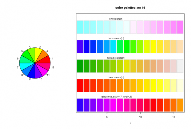
R Color Selection: Simple figure illustrating the layout() function to create a plot of the built-in R colors palettes.
Simple Color Display
#make a color wheel
pie(rep(1,12), col=rainbow(12))


#make a list of the common color palettes:
demo.pal <- function(n, border = if (n<32) "light gray" else NA,
main = paste("color palettes;  n=",n),
ch.col = c("rainbow(n, start=.7, end=.1)", "heat.colors(n)",
"terrain.colors(n)", "topo.colors(n)", "cm.colors(n)"))
{
        nt <- length(ch.col)
        i <- 1:n; j <- n / nt; d <- j/6; dy <- 2*d
        plot(i,i+d, type="n", yaxt="n", ylab="", main=main)
        for (k in 1:nt) {
                rect(i-.5, (k-1)*j+ dy, i+.4, k*j,
                        col = eval(parse(text=ch.col[k])), border = border)
                text(2*j,  k * j +dy/4, ch.col[k])
        }
}
n <- if(.Device == "postscript") 64 else 16
        # Since for screen, larger n may give color allocation problem
demo.pal(n)
A Queryable color picker (as suggested by Gabor Grothendieck on the R-help mailing list)
#make a color lookup function
getColorName <- function(colorNumber) colors()[colorNumber]

# pch = NA means no points plotted.  pch = 20 plots small dots.
# n is the number of points to identify interactively with mouse
printColorSampler <- function(n = 0, pch = NA, bg = "white") {
   i <- seq(colors())
   k <- ceiling(sqrt(length(i)))
   xy <- cbind(floor(i/k)*2, i %% k)
   opar <- par(bg = bg)
   on.exit(par = opar)
   plot(xy, axes = FALSE, xlab = "", ylab = "", pch=pch, col=colors())
   text(xy[,1]+.5, xy[,2]+.2, i, col = colors(), cex = 0.7)
   if (n > 0)
      colors()[identify(xy, n = n, labels = colors(), plot = FALSE)]
}

# test
printColorSampler(0)
printColorSampler(1)
printColorSampler(pch=20, bg="black")
Setup the plot layout, and plot both examples
#setup the layout, and print pane boundaries:
nf <- layout(matrix(c(1,1,2,2), 2, 2, byrow=FALSE), respect=TRUE, widths=c(1,2)) ; layout.show(nf)

#plot the pie chart:
pie(rep(1,12), col=rainbow(12))
#plot the palette chart:
demo.pal(n)

#save a copy to an EPS file:
dev.copy2eps()
