
Raster profile along arbitrary line segments
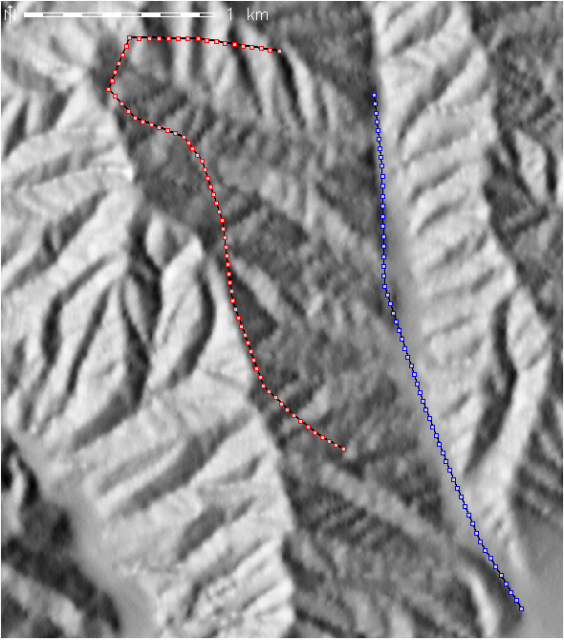
Sample profile creation I: Vector
representation of 2 transects
performed by an adventurous soil
scientist near McCabe Canyon,
Pinnacles National Monument.
Overview
A simple experiment illustrating the calculation of elevation profiles along arbitrary line segments using a combination of GRASS and R. Fractal dimension was calculated for each profile by spectral decomposition (FFT), as suggested in (Davis, 2002). Note that the elevation profiles are calculated in a rather non-standard way, as elevation is plotted against 3D distance along the original line segment. This means that resulting transect lengthcalculations are sensitive to the resolution of the raster (or distance between sample points), across a rough surface: i.e. smaller grid spacing will result in a longer effective (3D) transect length.
References
- Davis, J.C. Statistics and Data Analysis in Geology John Wiley and Sons, 2002
Create 2 profiles in GRASS
 # digitize some new lines in an area of interest
v.digit -n map=valley bgcmd="d.rast elev_meters"
v.digit -n map=mtns bgcmd="d.rast elev_meters"

# convert to points
v.to.points -i -v -t in=valley out=valley_pts type=line dmax=50
v.to.points -i -v -t in=mtns out=mtns_pts type=line dmax=50

# set resolution to match DEM
g.region -pa res=4

# extract elevation at each point
v.drape in=valley_pts out=valley_pts_3d type=point rast=elev_4m method=cubic
v.drape in=mtns_pts out=mtns_pts_3d type=point rast=elev_4m method=cubic

# export to text files
v.out.ascii valley_pts_3d > valley_pts_3d.txt
v.out.ascii mtns_pts_3d > mtns_pts_3d.txt

# start R
R
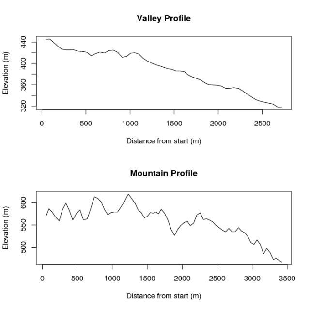
Sample profile creation II: Elevation profiles for the paths taken by the soil scientist here.
Process profile data, and plot in R
# read in the data, note that there is no header, and the columns are pipe delimited
valley <- read.table('valley_pts_3d.txt', header=F, sep="|", col.names=c('easting','northing','elev','f'))
mtns <- read.table('mtns_pts_3d.txt', header=F, sep="|", col.names=c('easting','northing','elev','f'))


# compute the length minus 1 ; i.e. the number of points - 1
# use for the lagged distance calculation
s.valley <- length(valley$easting) - 1
s.mtns <- length(mtns$easting) - 1

# calculate the lagged distance along each component of the 3D vector
dx.valley <- valley$easting[2:(s.valley+1)] - valley$easting[1:s.valley]
dy.valley <- valley$northing[2:(s.valley+1)] - valley$northing[1:s.valley]
dz.valley <- valley$elev[2:(s.valley+1)] - valley$elev[1:s.valley]

dx.mtns <- mtns$easting[2:(s.mtns+1)] - mtns$easting[1:s.mtns]
dy.mtns <- mtns$northing[2:(s.mtns+1)] - mtns$northing[1:s.mtns]
dz.mtns <- mtns$elev[2:(s.mtns+1)] - mtns$elev[1:s.mtns]

# combine the vector components
# 3D distance formula
c.valley <- sqrt( dx.valley^2 + dy.valley^2 + dz.valley^2)
c.mtns <- sqrt( dx.mtns^2 + dy.mtns^2 + dz.mtns^2)

# create the cumulative distance along line:
dist.valley <- cumsum(c.valley[1:s.valley])
dist.mtns <- cumsum(c.mtns[1:s.mtns])

# plot the results
par(mfrow=c(2,1))
plot(dist.valley, valley$elev[1:s.valley], type='l', xlab='Distance from start (m)', ylab='Elevation (m)', main='Profile')
plot(dist.mtns, mtns$elev[1:s.mtns], type='l', xlab='Distance from start (m)', ylab='Elevation (m)', main='Profile')
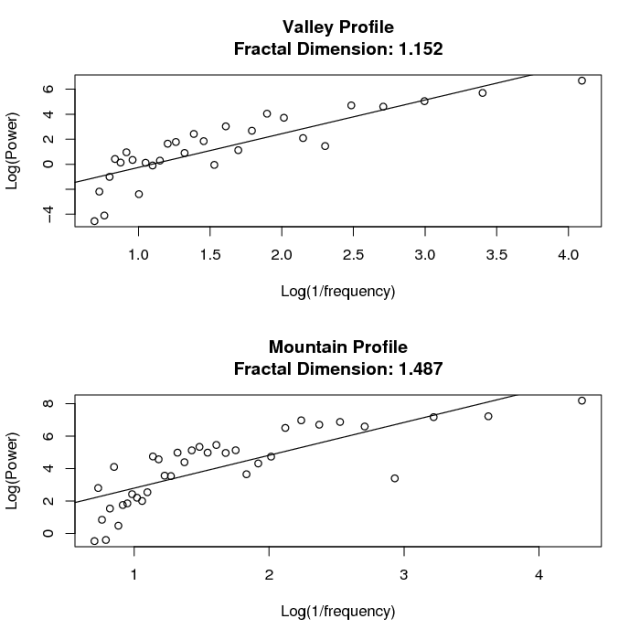
Sample profile creation III: Spectral decomposition (by FFT) for each profile.
Compute fractal dimension of each transect by FFT
 #compute the fractal dimension via [1]
s.valley <- spectrum(valley$elev[1:s.valley])
s.mtns <- spectrum(mtns$elev[1:s.mtns])

# compute linear model of log(power) ~ log(1/frequency)
# use the slope estimate in [2]

# first define the model formuals: for plotting and for lm()
fm.valley <- log(s.valley$spec) ~ log(1/s.valley$freq)
fm.mtns <- log(s.mtns$spec) ~ log(1/s.mtns$freq)

# next compute the least-squares regression lines via lm()
lm.valley <- lm(fm.valley)
lm.mtns <- lm(fm.mtns)

# extract the slope of each regression line:
slope.valley <- coef(lm.valley)[2]
slope.mtns <- coef(lm.mtns)[2]

# compute Df - the fractal dimension from [3]
Df.valley <- (5 - slope.valley) / 2
Df.mtns <- (5 - slope.mtns) / 2

# plot the figures
plot(fm.valley, main=paste("Valley Profile\nFractal Dimension: ", round(Df.valley,3), sep=''), xlab='Log(1/frequency)', ylab='Log(Power)' )
abline(lm.valley)

plot(fm.mtns, main=paste("Mountain Profile\nFractal Dimension: ", round(Df.mtns,3), sep=''), xlab='Log(1/frequency)',  ylab='Log(Power)')
abline(lm.mtns)
