
Premise
Small update to a similar thread from last week, on the comparison of slope and intercept terms fit to a multi-level model. I finally figured out (thanks R-Help mailing list!) how to efficiently use contrasts in R. The C() function can be called within a model formula, to reset the base level of an un-ordered factor. The UCLA Stats Library has an extensive description of this topic here. This approach can be used to sequentially test for differences between slope and intercept terms from a multi-level model, by re-setting the base level of a factor. See example data and figure below.
Note that the multcomp package has a much more robust approach to this type of operation. Details below.
Example Multi-Level Data
# need these
library(lattice)
# replicate an important experimental dataset
set.seed(10101010)
x <- rnorm(100)
y1 <- x[1:25] * 2 + rnorm(25, mean=1)
y2 <- x[26:50] * 2.6 + rnorm(25, mean=1.5)
y3 <- x[51:75] * 2.9 + rnorm(25, mean=5)
y4 <- x[76:100] * 3.5 + rnorm(25, mean=5.5)
d <- data.frame(x=x, y=c(y1,y2,y3,y4), f=factor(rep(letters[1:4], each=25)))
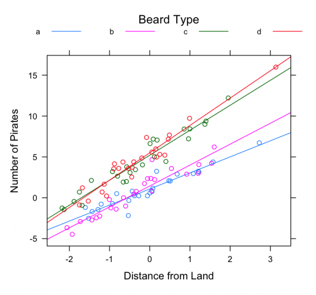
# plot
xyplot(y ~ x, groups=f, data=d,
auto.key=list(columns=4, title='Beard Type', lines=TRUE, points=FALSE, cex=0.75),
type=c('p','r'), ylab='Number of Pirates', xlab='Distance from Land')
Example Multi-Level Model II
Default Contrasts (contr.treatment for regular factors, contr.poly for ordered factors)
# standard comparison to base level of f
summary(lm(y ~ x * f, data=d))

# output:
Coefficients:
            Estimate Std. Error t value Pr(>|t|)
(Intercept)   1.0747     0.1889   5.689 1.51e-07 ***
x             1.9654     0.1799  10.927  < 2e-16 ***
fb            0.3673     0.2724   1.348   0.1808
fc            4.1310     0.2714  15.221  < 2e-16 ***
fd            4.4309     0.2731  16.223  < 2e-16 ***
x:fb          0.5951     0.2559   2.326   0.0222 *
x:fc          1.0914     0.2449   4.456 2.35e-05 ***
x:fd          1.3813     0.2613   5.286 8.38e-07 ***
---
Signif. codes:  0 ‘***’ 0.001 ‘**’ 0.01 ‘*’ 0.05 ‘.’ 0.1 ‘ ’ 1
Setting the "base level" in the Model Formula This allows us to compare all slope and intercept terms to the slope and intercept from level 4 of our factor ('d' in our example).
# compare to level 4 of f
summary(lm(y ~ x * C(f, base=4), data=d))

# output:
Coefficients:
                  Estimate Std. Error t value Pr(>|t|)
(Intercept)         5.5055     0.1972  27.911  < 2e-16 ***
x                   3.3467     0.1896  17.653  < 2e-16 ***
C(f, base = 4)1    -4.4309     0.2731 -16.223  < 2e-16 ***
C(f, base = 4)2    -4.0635     0.2783 -14.603  < 2e-16 ***
C(f, base = 4)3    -0.2999     0.2773  -1.081  0.28230
x:C(f, base = 4)1  -1.3813     0.2613  -5.286 8.38e-07 ***
x:C(f, base = 4)2  -0.7862     0.2628  -2.992  0.00356 **
x:C(f, base = 4)3  -0.2899     0.2521  -1.150  0.25327
---
Signif. codes:  0 ‘***’ 0.001 ‘**’ 0.01 ‘*’ 0.05 ‘.’ 0.1 ‘ ’ 1
Testing with Multcomp Package using data from above example
# need these
library(multcomp)
library(sandwich)

# open this vignette, lots of good information
vignette("generalsiminf", package = "multcomp")

# fit two models
l.1 <- lm(y ~ x + f, data=d)
l.2 <- lm(y ~ x * f, data=d)

# note that: tests are AGAINST the null hypothesis
summary(glht(l.1))

# see the plotting methods:
plot(glht(l.1))
plot(glht(l.2))

# pair-wise comparisons
summary(glht(l.1, linfct=mcp(f='Tukey')))

# pair-wise comparisons
# may not be appropriate for model with interaction
summary(glht(l.2, linfct=mcp(f='Tukey')))

# when variance is not homogenous between groups:
summary(glht(l.1, linfct=mcp(f='Tukey'), vcov=sandwich))
Links:
Comparison of Slope and Intercept Terms for Multi-Level Model
R: advanced statistical package
Computing Statistics from Poorly Formatted Data (plyr and reshape packages for R)
