
Finally made it out to Folsom Lake for a fine day of sailing and GPS track collecting. Once I was back in the lab, I downloaded the track data with gpsbabel, and was ready to import the data into GRASS.
# import GPX from GPS:
gpsbabel -t -i garmin -f /dev/ttyS0 -o gpx -F trip1.gpx
I was particularly interested in how fast we were able to get the boat going, however my GPS does not keep track of its speed in the track log. Also, I had forgotten to set GPS up for a constant time interval between track points. Dang. In order to compute a velocity between sequential points from the track log I would need to first do two things: 1) convert the geographic coordinates into projected coordinates, and 2) compute the associated time interval between points.
The GDAL/OGR tools provide one of the simplest means of simultaneously converting between formats AND coordinate systems. The GPX file contains both a line and point representation of the log; the point version seems simpler to work with. Initially I used the default output format (ESRI shapefile), however I quickly discovered that the datetime information from the GPX file was silently truncated to just the date part. Turns out that GDAL/OGR can now write vector data inSQLite format-- storing both the geometry and attributes into a single file, with a table structure very similar to PostGIS. Seems like a great replacement for shapefiles, that can deal with complex data types, long field names, and probably very large geometries.
# convert into sqlite DB with geometry-- better preservation of attributes
ogr2ogr -F "SQLite" -t_srs '+proj=utm +zone=10 +datum=NAD83' trip1_track_points.db trip1.gpx track_points

# import, we are using a sqlite DB back-end
v.in.ogr dsn=trip1_track_points.db out=folsom_trip1_pts
Next, we import the data (in projected coordinates) into a GRASS location/mapset, with a SQLite database back-end. The data are now in a format that can be easily imported into R for velocity calculations, and then sent back to GRASS for further processing. An example R session is presented below. Track points are in chronological order, so we can use the diff() function for computing sequential time and distance intervals.
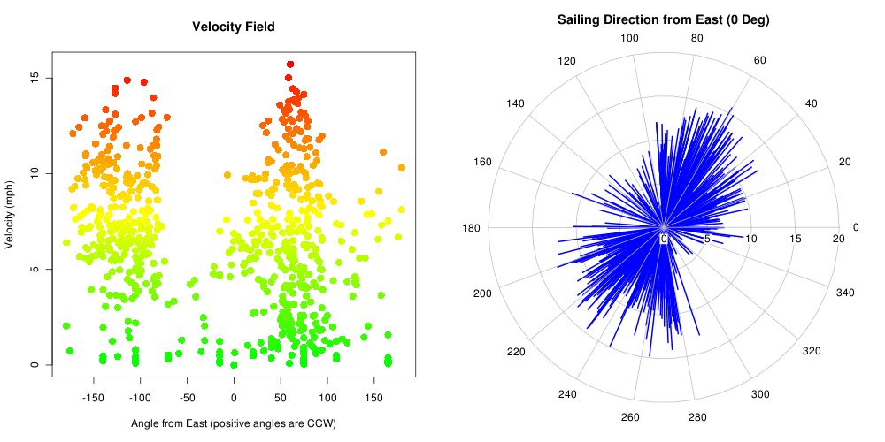
Figure: Velocity vs. Bearing
Further rocessing in R
library(spgrass6)
library(RColorBrewer)
library(plotrix)


# read vector points
# alternatively we probably could have read in the GPX format directly
x <- readVECT6('folsom_trip1_pts')

# convert date/time field
x@data$date_time <- as.POSIXct(strptime(x@data$time, format="%Y/%m/%d %H:%M:%S+00"))

# distance intervals (meters)
dx <- diff(x@coords[,1])
dy <- diff(x@coords[,2])
x.dist <- sqrt(dx^2 + dy^2)

# time interval (seconds)
x.dt <- diff(x@data$date_time)

# compute velocity and convert to mph
x.meters_per_second <- x.dist / as.numeric(x.dt)
x.mph <- x.meters_per_second * 2.2369

# compute bearing
x.bearing <- atan2(dy, dx) * 180/pi

# add back to original DF
# note that first point has no velocity or bearing
x@data$mph <- NA
x@data$bearing <- NA
x@data$mph[-1] <- x.mph
x@data$bearing[-1] <- x.bearing

# check visually
spplot(x, 'mph', col.regions=brewer.pal('Spectral', n=5), cuts=5)
spplot(x, 'bearing', col.regions=brewer.pal('Spectral', n=5), cuts=5)

# keep only interesting information in the attribute table
# note that this destroys the original object's table
x@data <- x@data[, c('cat','ele','time','date_time','mph','bearing')]

# save data back to GRASS
writeVECT6(x, 'folsom_trip1_pts_dt')

# fancy plots
png(file='speed_vs_bearing.png', width=1000, height=500)
par(mfcol=c(1,2))
plot(mph ~ bearing, data=x@data, xlim=c(-180,180), xlab="Angle from East (positive angles are CCW)",
ylab="Velocity (mph)", main="Velocity Field", col=color.scale(mph,c(0,1,1),c(1,1,0),0), pch=16, cex=1.5)

## polar plot:
polar.plot(x@data$mph[-1], x@data$bearing[-1] ,main="Sailing Direction from East (0 Deg)", line.col='blue', lwd=2)
dev.off()
