
Dendrograms are a convenient way of depicting pair-wise dissimilarity between objects, commonly associated with the topic of cluster analysis. This is a complex subject that is best left to experts and textbooks, so I won't even attempt to cover it here. I have been frequently using dendrograms as part of my investigations into dissimilarity computed between soil profiles. Unfortunately the interpretation of dendrograms is not very intuitive, especially when the source data are complex. In addition, pair-wise dissimimlarity computed between soil profiles and visualized via dendrogram should not be confused with the use of dendrograms in the field of cladistics-- where relation to a common ancestor is depicted.
An example is presented below that illustrates the relationship between dendrogram and dissimilarity as evaluated between objects with 2 variables. Essentially, the level at which branches merge (relative to the "root" of the tree) is related to their similarity. In the example below it is clear that (in terms of clay and rock fragment content) soils 4 and 5 are more similar to each other than to soil 2. In addition, soils 1 and 3 are more similar to each other than soils 4 and 5 are to soil 2. Recall that in this case pair-wise dissimilarity is based on the Euclidean distance between soils in terms of their clay content and rock fragment content. Therefore proximity in the scatter plot of frock frags vs. clay is directly related to our simple evaluation of "dissimilarity". Inline-comments in the code below elaborate further.
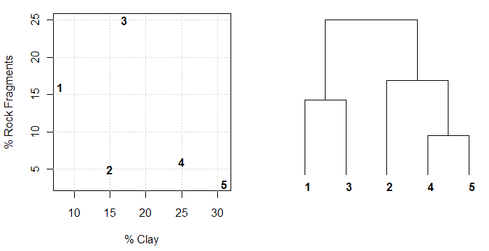
Image: Data to Dendrogram
Example Code
# load required libraries
library(cluster) # clustering functions
library(ape) # nicer plotting of dendrograms

# simulate some aggregate profile data
frags <- c(16, 5, 25, 6, 3) # rock fragments
clay <- c(8, 15, 17, 25, 31) # clay contents

# combine into single data.frame
s <- data.frame(clay, frags)

# evaluate pair-wise dissimilarity based on clay and frag %
# since both measurements are on the same scale, no standardization is needed
d <- daisy(s)

# inspect pair-wise dissimilarity matrix
print(d)

# perform divisive hierarcical clustering for dendrogram creation
d.diana <- diana(d)

# convert object into 'phylo' class for plotting
d.phylo <- as.phylo(as.hclust(d.diana))

# 2-figure plot of original data and resulting dendrogram repsesentation of dissimilarity matrix
par(mfcol=c(1,2), mar=c(4.5,4,1,1))
# original data: setup plot, but don't actually plot it
plot(frags ~ clay, data=s, type='n', xlab='% Clay', ylab='% Rock Fragments')
# add grid lines to assist the eye
grid()
# annotate empty plot with soil numbers
text(s$clay, s$frags, row.names(s), font=2)

# plot dendrogram representation, annotated with the same labels
plot(d.phylo, font=2, label.offset=1, direction='down', srt=90)
