
Continuing the previous discussion of pair-wise dissimilarity between soil profiles, the following demonstration (code, comments, and figures) further elaborates on the method. A more in-depth discussion of this example will be included as a vignette within the 1.0 release of AQP.
Total, Between-Profile Dissimilarity
# setup environment
library(aqp)
library(ape)
library(RColorBrewer)
library(latticeExtra)
library(plotrix)
# setup some colors
cols <- brewer.pal(3, 'Set1')
# setup horizon-level data: data are from lab sampled pedons
d <- structure(
list(
series = c("auburn", "auburn", "auburn", "auburn", "dunstone", "dunstone", "dunstone", "dunstone", "sobrante", "sobrante", "sobrante", "sobrante", "sobrante"),
top = c(0, 3, 15, 25, 0, 5, 17, 31, 0, 5, 10, 28, 51),
bottom = c(3, 15, 25, 47, 5, 17, 31, 41, 5, 10, 28, 51, 74),
clay = c(21, 21, 20, 21, 16, 17, 20, 21, 18, 16, 15, 18, 20),
frags = c(6, 13, 9, 28, 13, 19, 6, 15, 0, 2, 21, 13, 12),
ph = c(5.6, 5.6, 5.8, 5.8, 6, 6.3, 6.3, 6.3, 5.8, 5.7, 5.8, 6.2, 6.2)
),
.Names = c("series", "top", "bottom", "clay", "frags", "ph"),
row.names = c(NA, -13L),
class = "data.frame"
)
# establish site-level data
s <- data.frame(
series=c('auburn', 'dunstone', 'sobrante'),
precip=c(24, 30, 32),
stringsAsFactors=FALSE
)
# generate fake horizon names with clay / frags / ph
d$name <- with(d, paste(clay, frags, ph, sep='/'))
# upgrade to SoilProfile Collection object
depths(d) <- series ~ top + bottom
site(d) <- s
# inspect variables used to determine dissimilarity
cloud(clay ~ ph + frags, groups=series, data=horizons(d), auto.key=list(columns=3, points=TRUE, lines=FALSE), par.settings=list(superpose.symbol=list(pch=16, col=cols, cex=1.5)))
# compute betwee-profile dissimilarity, no depth weighting
d.dis <- profile_compare(d, vars=c('clay', 'ph', 'frags'), k=0, max_d=61, replace_na=TRUE, add_soil_flag=TRUE)
# check total, between-profile dissimilarity, normalized to maximum
d.m <- signif(as.matrix(d.dis / max(d.dis)), 2)
print(d.m)
# group via divisive hierarchical clustering
d.diana <- diana(d.dis)
# convert classes, for better plotting
d.phylo <- as.phylo(as.hclust(d.diana))
# plot: 2 figures side-by-side
par(mfcol=c(1,2))
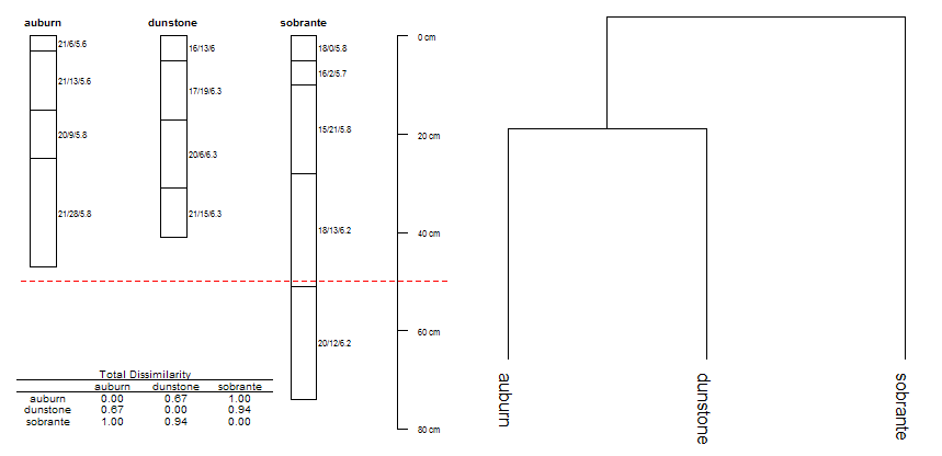
# profiles
plot(d, width=0.1, name='name')
# annotate shallow-mod.deep break
abline(h=50, col='red', lty=2)
# add dissimilarity matrix
addtable2plot(0.8, 70, format(d.m, digits=2), display.rownames=TRUE, xjust=0, yjust=0, cex=0.6, title='Total Dissimilarity')
# plot dendrogram in next panel
plot(d.phylo, direction='down', srt=0, font=1, label.offset=1)
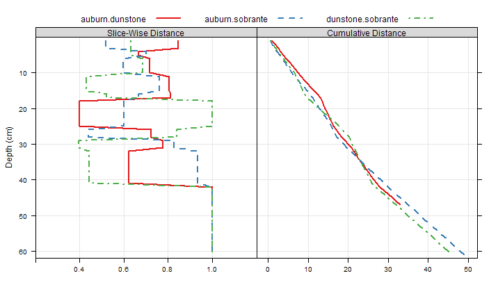
Image: Profile Dissimilarity Demo: MVO Soils, Slice-Wise Dissimilarity
Slice-wise, Between-Profile Dissimilarity
# continuing from example above...

# return dissimilarity matrices at each depth slice
d.dis.all <- profile_compare(d, vars=c('clay', 'ph', 'frags'), k=0, max_d=61, replace_na=TRUE, add_soil_flag=TRUE, return_depth_distances=TRUE)

# check between-profile dissimilarity, at slice 1
print(as.matrix(d.dis.all[[1]]))

# init functions for extracting pair-wise dissimilarity:
f.12 <- function(i) as.matrix(i)[1, 2] # between auburn and dunstone
f.13 <- function(i) as.matrix(i)[1, 3] # between auburn and sobrante
f.23 <- function(i) as.matrix(i)[2, 3] # between dunstone and sobrante

# apply functions at each slice
d.12 <- sapply(d.dis.all, f.12)
d.13 <- sapply(d.dis.all, f.13)
d.23 <- sapply(d.dis.all, f.23)

# combine into single data.frame
d.all <- make.groups(
        auburn.dunstone=data.frame(slice=1:61, d=d.12, d.sum=cumsum(d.12)),
        auburn.sobrante=data.frame(slice=1:61, d=d.13, d.sum=cumsum(d.13)),
        dunstone.sobrante=data.frame(slice=1:61, d=d.23, d.sum=cumsum(d.23))
        )

# plot slice-wise dissimilarity between all three soils
p.1 <- xyplot(slice ~ d, groups=which, data=d.all, ylim=c(62,0), type=c('l','g'), xlim=c(0.2,1.2), ylab='Depth (cm)', xlab='', horizontal=TRUE, auto.key=list(columns=3, lines=TRUE, points=FALSE), asp=1)

# plot slice-wise, cumulative dissimilarity between all three soils
p.2 <- xyplot(slice ~ d.sum, groups=which, data=d.all, ylim=c(62,0), type=c('l','g'), ylab='Depth (cm)', xlab='', horizontal=TRUE, auto.key=list(columns=3, lines=TRUE, points=FALSE), asp=1)

# combine into panels of a single figure
p.3 <- c('Slice-Wise Distance'=p.1, 'Cumulative Distance'=p.2)
# setup plotting style
trellis.par.set(superpose.line=list(col=cols, lwd=2, lty=c(1,2,4)), strip.background=list(col=grey(0.85)))
# render figure
print(p.3)
