
UPDATE 2013-04-08: This functionality is now available in the sharpshootRpackage.
Previously, soil profile comparison methods from the aqp package only took into account horizon-level attributes. As of last week the profile_compare() function can now accommodate horizon and site-level attributes. In other words, it is now possible to compute pair-wise dissimilarity between soil profiles using a combination of horizon-level properties (soil texture, pH, color, etc.) and site-level properties (surface slope, vegetation, soil taxonomy, etc.)-- continuous, categorical, or boolean.
An example is presented below which is based on the loafercreek sample data set included with the soilDB package. Be sure to use the latest version of soilDB, 0.5-5 or later. Dissimilarity matrices created from horizon and site+horizon data are compared by placing their respective dendrograms back-to-back. Code from the ape package is used to facilitate dendrogram plotting, manipulation, and indexing. Blue line segments connect matching nodes from each dendrogram. Soil profiles with paralithic contact are marked with orange squares for clarity.
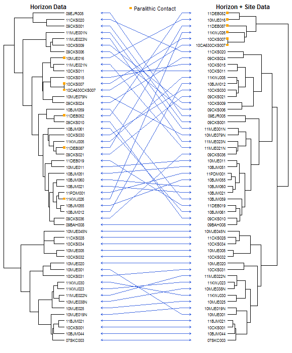
Image: Dueling Dendrograms
Example Code
# setup environment
library(soilDB)
library(cluster)
library(ape)

# load sample dataset from soilDB package
data(loafercreek)

# compare profiles with hz-level data only: need at least 2 variables
d.hz <- profile_compare(loafercreek, vars=c('clay', 'total_frags_pct'), k=0, max_d=100, rescale.result=TRUE)

# hz and site level variables: need at least 2 hz-level and 2 site-level
# character-class variables should be manually converted to factors first
d.site.hz <- profile_compare(loafercreek, vars=c('clay', 'total_frags_pct', 'paralithic.contact', 'slope'), k=0, max_d=100, rescale.result=TRUE)

# verify: both dissimilarity matrices have been rescaled to [0,1]
range(d.hz) ; range(d.site.hz)

# cluster via divisive hierarchical algorithm
# convert to 'phylo' class
phylo.hz <- as.phylo(as.hclust(diana(d.hz)))
phylo.site.hz <- as.phylo(as.hclust(diana(d.site.hz)))

# generate vector of labels for site-level clustering criteria
# paralithic contact = 1, missing = 2
paralithic.contact.code <- as.integer(loafercreek$paralithic.contact)+1

# setup some geometry for connecting lines / arrows
arrow.left <- 0.1
arrow.right <- 0.9
arrow.length <- 0.1

# setup plot layout
lo <- layout(matrix(c(1,3,2), ncol=3), widths=c(1, 1, 1)) # check with: layout.show(lo)

# plot hz-level dissimilarities on left-hand side
plot(phylo.hz, cex=0.75, font=1, no.margin=TRUE, direction='rightwards', label.offset=0.015)
mtext('Horizon Data', side=3, line=-1.5, font=2, cex=0.75)

# save results of phylo environment
p.left <- get("last_plot.phylo", envir = .PlotPhyloEnv)
# annotate pedons with paralithic contact
tiplabels(pch=15, col=c('orange', NA)[paralithic.contact.code])

# plot site+hz-level dissimilarities on right-hand side
plot(phylo.site.hz, cex=0.75, font=1, direction='leftwards', no.margin=TRUE, label.offset=0.015)
mtext('Horizon + Site Data', side=3, line=-1.5, font=2, cex=0.75)

# save results of phylo environment
p.right <- get("last_plot.phylo", envir = .PlotPhyloEnv)
# annotate pedons with paralithic contact
tiplabels(pch=15, col=c('orange', NA)[paralithic.contact.code])

# get ordering of pedon IDs on each side
# left-hand side
left.new_order <- sapply(1:p.left$Ntip, function(i) which(as.integer(p.left$yy[1:p.left$Ntip]) == i))
# right-hand side
right.new_order <- sapply(1:p.right$Ntip, function(i) which(as.integer(p.right$yy[1:p.right$Ntip]) == i))

# re-order right-hand side nodes so that they match the ordering of left-side nodes
left.right.converstion.order <- right.new_order[match(left.new_order, right.new_order)]

# setup new plot region
par(mar=c(0,0,0,0))
plot(0, 0, type='n', xlim=c(0,1), ylim=range(p.left$yy), axes=FALSE, xpd=FALSE)

# plot connecting segments
segments(x0=arrow.left, y0=p.left$yy[left.new_order], x1=arrow.right,
y1=p.right$yy[left.right.converstion.order], col='RoyalBlue')

# plot helper arrows
arrows(x0=arrow.left, y0=p.left$yy[left.new_order], x1=arrow.left-arrow.length, y1=p.left$yy[left.new_order], col='RoyalBlue', code=2, length=0.05)
arrows(x0=arrow.right, y0=p.right$yy[right.new_order], x1=arrow.right+arrow.length, y1=p.right$yy[right.new_order], col='RoyalBlue', code=2, length=0.05)

# legend: top-center
legend('top', legend=c('Paralithic Contact'), pch=15, col='orange', bty='n')
