
UPDATED 2013-04-08
This functionality it now available in the soilDB and sharpshootR packages. All code on this page is now superseded by the fetchOSD() and SoilTaxonomyDendrogram()functions.
UPDATED 2012-11-07
I have been thinking about a URL-based interface to basic Official Soil Series Description (OSD) data for a while now... something that when fed a URL, would return CSV-formatted records to the calling process. These type of interfaces can later be used to support more complicated systems, such as our smartphone interface to SoilWeb. URLs can be accessed like files in R, making it possible to do something like this:
OSD Site-Level Data
read.csv(url('casoilresource.lawr.ucdavis.edu/soil_web/reflector_api/soils.php?what=osd_site_query&q_string=auburn,sobrante'))

# returning:
seriesname,soilorder,suborder,grtgroup,subgroup_mod
AUBURN,INCEPTISOLS,XEREPTS,HAPLOXEREPTS,LITHIC
SOBRANTE,ALFISOLS,XERALFS,HAPLOXERALFS,MOLLIC
OSD Horizon-Level Data
read.csv(url('casoilresource.lawr.ucdavis.edu/soil_web/reflector_api/soils.php?what=osd_query&q_string=auburn,sobrante'))

# returning:
series,layer,name,top,bottom,matrix_dry_color_hue,matrix_dry_color_value,matrix_dry_color_chroma,matrix_wet_color_hue,matrix_wet_color_value,matrix_wet_color_chroma,texture,cfrags
AUBURN,1,A1,0,4,7.5YR,5,6,5YR,4,4,silt loam,
AUBURN,2,A2,4,23,5YR,5,6,5YR,4,4,silt loam,
AUBURN,3,Bw,23,36,5YR,5,8,5YR,4,6,silt loam,
AUBURN,4,R,36,61,,,,,,,,
SOBRANTE,1,A,0,13,5YR,5,4,5YR,3,4,silt loam,
SOBRANTE,2,Bt1,13,28,5YR,4,6,5YR,3,6,silt loam,
SOBRANTE,3,Bt2,28,61,5YR,5,6,2.5YR,3,6,light clay loam,
SOBRANTE,4,Cr,61,76,,,,,,,,
SOBRANTE,5,R,76,86,,,,,,,,
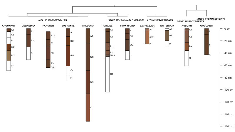
Simple access to basic OSD site and horizon-level data makes it possible to rapidly assemble OSD data within R. For example, multiple soil profile sketches, based on OSD data, can be quickly arranged into a figure according to their taxonomic membership. With pair-wise dissimilarities computed from categorical variables, cluster analysis reduces to an elegant sorting method and depicted as a dendrogram. Between-profile similarity can be determined graphically, with soils sharing the same taxonomic membership placed along the same terminal branches. In the example below, parent material information, soil depth class, or any number of horizon-level attributes could be combined with the site parameters for a more relevant grouping. The following code could use some clean-up and heuristics for automatically determining some of the fudge factors used to position elements within the figure. Also, it would be nice to annotate branches associated with suborder and greatgroup membership. I'll save that for next time.
Note that these data are a snapshot of the OSD database-- as of a couple years ago. Therefore, recently established soil series are missing, and changes may have been made to existing series since then. Please use these links with this in mind.
Implementation
# need these
library(aqp)
library(cluster)
library(ape)

# soils of interest
s.list <- c('san joaquin','montpellier','grangeville','pollasky','ramona')

# base URLs
u.osd_site <- 'http://casoilresource.lawr.ucdavis.edu/soil_web/reflector_api/soils.php?what=osd_site_query&q_string='
u.osd_hz <- 'http://casoilresource.lawr.ucdavis.edu/soil_web/reflector_api/soils.php?what=osd_query&q_string='

# compile URL + requested soil series
u.site <- paste(u.osd_site, paste(s.list, collapse=','), sep='')
u.hz <- paste(u.osd_hz, paste(s.list, collapse=','), sep='')

# request data
s <- read.csv(url(u.site), stringsAsFactors=TRUE)
h <- read.csv(url(u.hz), stringsAsFactors=FALSE)

# reformatting and color conversion
h$soil_color <- with(h, munsell2rgb(matrix_wet_color_hue, matrix_wet_color_value, matrix_wet_color_chroma))
h <- with(h, data.frame(id=series, top, bottom, hzname, soil_color,
                                                                                                hue=matrix_wet_color_hue, value=matrix_wet_color_value,
                                                                                                chroma=matrix_wet_color_chroma, stringsAsFactors=FALSE))

# upgrade to SoilProfileCollection
depths(h) <- id ~ top + bottom

# plot profiles
par(mar=c(0,0,0,0))
plot(h, name='hzname', cex.names=0.85, axis.line.offset=-4)

# compute dissimilarity via subgroup classification
# cluster using divisive algorithm
h.hclust <- as.hclust(diana(s[, c(2,3,4,5)]))

# add series name as labels
h.hclust$labels <- s$series

# convert to phylo class
p <- as.phylo(h.hclust)

# plot profiles below corresponding leaves in the dendrogram
par(mar=c(0,0,0,0))
plot(p, cex=0.8, direction='up', y.lim=c(20,0), x.lim=c(0.5, length(h)+1), show.tip.label=FALSE)

# get the last plot geometry
lastPP <- get("last_plot.phylo", envir = .PlotPhyloEnv)

# vector of indices for plotting soil profiles below leaves of dendrogram
new_order <- sapply(1:lastPP$Ntip, function(i) which(as.integer(lastPP$xx[1:lastPP$Ntip]) == i))

# plot the profiles, in the ordering defined by the dendrogram
# with a couple fudge factors to make them fit
plot(h, name='hzname', plot.order=new_order, max.depth=150, n.depth.ticks=6, scaling.factor=0.1, cex.names=0.75, cex.id=0.75, axis.line.offset=-4, width=0.1, y.offset=max(lastPP$yy) + 1.5, add=TRUE)

# generate taxonomic labels and their positions under the dendrogram
lab <- s[new_order, 'subgroup']
unique.lab <- unique(lab)
group.lengths <- rle(as.numeric(lab))$lengths
lab.positions <- (cumsum(group.lengths) - (group.lengths / 2)) + 0.5

# add labels-- note manual tweaking of y-coordinates
text(lab.positions, 2.6, unique.lab, cex=0.75, adj=0.5, font=4)
