
R provides several frameworks for composing figures. Base graphics is the simplest, grid is more advanced, and the lattice/ggplot packages provide convenient abstractions of the grid graphics system. Multi-element figures can be readily created in base graphics using either par() or layout(), with analogous functions available in grid. Mixing the two systems is a little more complicated, somewhat fragile, but entirely possible.
I recently needed to combine base+grid graphics on a single page; two sets of base graphics on the left, and the output from xyplot() (grid) on the right. Following some tips from Paul Murrell posted on r-help, the solution was fairly simple. A truncated example of the processes is listed below, corresponding to the attached figure. While the result was "good enough" for a quick summary, there are clearly some improvements that would make figure more useful.
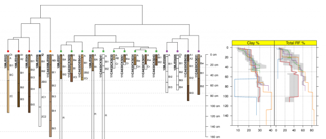
Image: Mehrten Soil Summary
Sample Code
# libraries
library(grid)
library(gridBase)
library(lattice)

# ... this is a truncated example ...

# start new page
par(mar=c(0,0,0,0), no.readonly=TRUE)
plot.new()

# setup layout
gl <- grid.layout(nrow=2, ncol=2, widths=unit(c(2,1), 'null'), heights=unit(c(1,3), 'null'))
# grid.show.layout(gl)

# setup viewports
vp.1 <- viewport(layout.pos.col=1, layout.pos.row=c(1,2)) # dend + profiles
vp.2 <- viewport(layout.pos.col=2, layout.pos.row=2) # depth functions

# init layout
pushViewport(viewport(layout=gl))
# access the first position
pushViewport(vp.1)

# start new base graphics in first viewport
par(new=TRUE, fig=gridFIG())

p.plot <- plot(p, cex=0.8, label.offset=-3, direction='up', y.lim=c(200,0),
x.lim=c(1, length(m)+1), show.tip.label=FALSE)
tiplabels(pch=15, col=cols[grps])

# get the last plot geometry
lastPP <- get("last_plot.phylo", envir = .PlotPhyloEnv)

# vector of indices for plotting soil profiles below leaves of dendrogram
new_order <- sapply(1:lastPP$Ntip,
  function(i) which(as.integer(lastPP$xx[1:lastPP$Ntip]) == i))

# plot the profiles, in the ordering defined by the dendrogram
# with a couple fudge factors to make them fit
sf <- 0.8
yoff <- max(lastPP$yy) + 5

# add lines at soil depth classes
dc <- c(25,50,75,100,150) * sf + yoff
abline(h=dc, lty=2, col='grey')

profile_plot(m, color="soil_color", plot.order=new_order, cex.id=0.75, max.depth=150,
n.depth.ticks=6, scaling.factor=sf, width=0.1, cex.names=0.65, cex.depth.axis=0.75,
y.offset=yoff, add=TRUE, name='hzname', id.style='side')

# done with the first viewport
popViewport()

# move to the next viewport
pushViewport(vp.2)

# print our lattice graphics here
print(p.1, newpage=FALSE)

# done with this viewport
popViewport(1)
