
Principal Coordinates (of) Neighbor Matrices (PCNM) is an interesting algorithm, developed by P. Borcard and P. Legendre at the University of Montreal, for the multi-scale analysis of spatial structure. This algorithm is typically applied to a distance matrix, computed from the coordinates where some environmental data were collected. The resulting "PCNM vectors" are commonly used to describe variable degrees of possible spatial structure and its contribution to variability in other measured parameters (soil properties, species distribution, etc.)-- essentially a spectral decomposition spatial connectivity. This algorithm has been recently updated by and released as part of the PCNM package for R. Several other implementations of the algorithm exist, however this seems to be the most up-to-date.
Related Presentations and Papers on PCNM
- http://biol09.biol.umontreal.ca/ESA_SS/Borcard_&_PL_talk.pdf
- Borcard, D. and Legendre, P. 2002. All-scale spatial analysis of ecological data by means of principal coordinates of neighbour matrices. Ecological Modelling 153: 51-68.
- Borcard, D., P. Legendre, Avois-Jacquet, C. & Tuomisto, H. 2004. Dissecting the spatial structures of ecologial data at all scales. Ecology 85(7): 1826-1832.
I was interested in using PCNM vectors for soils-related studies, however I encountered some in difficulty interpreting what they really meant when applied to irregularly-spaced site locations. As a demonstration, I generated several (25 to be exact) PCNM vectors from a regular grid of points. Using an example from the PCNM manual page, I have plotted the values of the PCNM vectors at the grid nodes (below). The interpretation of the PCNM vectors derived from a 2D, regular grid is fairly simple: lower order vectors represent regional-scale groupings, higher order vectors represent more local-scale groupings. One thing to keep in mind is that these vectors give us a multi-scale metric for grouping sites, and are not computed by any properties that may have been measured at the sites. The size of the symbols are proportional to the PCNM vectors and the color represents the sign.
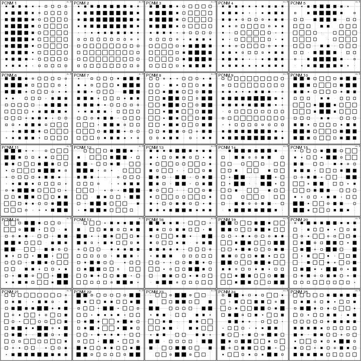
Figure: PCNM - Regular Grid
Soil survey operations are rarely conducted on a regular grid, so I re-computed PCNM vectors from the same simulated grid, but after randomly perturbing each site. The resulting map of PCNM vectors is presented below. The patterns are a little complex, but quickly decipherable with guidance from the PCNM vectors derived from a regular grid. Neat
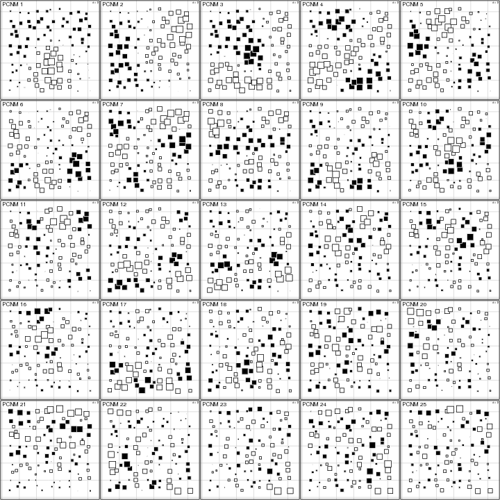
Figure: PCNM - Randomly Perturbed Regular Grid
R code used to make figures
library(ade4)
library(PCNM)

# fake data
g <- expand.grid(x=1:10, y=1:10)
x.coords <- data.frame(x=g$x, y=g$y)

# PCNM
x.sub.dist <- dist(x.coords[,c('x','y')])
x.sub.pcnm <- PCNM(x.sub.dist, dbMEM=TRUE)

# plot first 25 PCNM vectors
pdf(file='PCNM-grid-example.pdf', width=10, height=10)

par(mfrow=c(5,5))
for(i in 1:25)
        s.value(x.coords[,c('x','y')], x.sub.pcnm$vectors[,i], clegend=0, sub=paste("PCNM", i), csub=1.5, addaxes=FALSE, origin=c(1,1))

dev.off()


# jitter the same input and try again
x.coords <- data.frame(x=jitter(g$x, factor=2), y=jitter(g$y, factor=2))
x.sub.dist <- dist(x.coords[,c('x','y')])
x.sub.pcnm <- PCNM(x.sub.dist, dbMEM=TRUE)

# plot first 25 PCNM vectors
pdf(file='PCNM-jittered_grid-example.pdf', width=10, height=10)

par(mfrow=c(5,5))
for(i in 1:25)
        s.value(x.coords[,c('x','y')], x.sub.pcnm$vectors[,i], clegend=0, sub=paste("PCNM", i), csub=1.5, addaxes=FALSE, origin=c(1,1))

dev.off()
Links:
Target Practice and Spatial Point Process Models
Working with Spatial Data
Visualizing Random Fields and Select Components of Spatial Autocorrelation
