
I recently noticed the new latticeExtra page on R-forge, which contains many very interesting demos of new lattice-related functionality. There are strong opinions about the "best" graphics system in R (base graphics, grid graphics, lattice, ggplot, etc.)-- I tend to use base graphics for simple figures and lattice for depicting multivariate or structured data. The sp package defines classes for storing spatial data in R, and contains several useful plotting methods such as the lattice-based spplot(). This function, and back-end helper functions, provide a generalized framework for plotting many kinds of spatial data. However, sometimes with great abstraction comes great ambiguity-- many of the arguments that would otherwise allow fine tuning of the figure are buried in documentation for lattice functions. Examples are more fun than links to documentation, so I put together a couple of them below. They describe several strategies for placing and adjusting map legends-- either automatically, or manually added with the update() function. The last example demonstrates an approach for over-plotting 2 rasters. All of the examples are based on the meuse data set, from the gstat package.
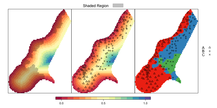
FIgure: Extended spplot() examples
Examples
# setup environment
library(gstat)
library(latticeExtra)
library(grid)

# load example data
data(meuse.grid)
data(meuse)
data(meuse.alt)

# convert to SpatialPointsDataFrame
coordinates(meuse.grid) <- ~ x + y
coordinates(meuse) <- ~ x + y
coordinates(meuse.alt) <- ~ x + y

# converto SpatialPixelsDataFram
gridded(meuse.grid) <- TRUE

# convert 'soil' to factor and re-label
meuse.grid$soil <- factor(meuse.grid$soil, labels=c('A','B','C'))
meuse$soil <- factor(meuse$soil, levels=c('1','2','3'), labels=c('A','B','C'))


#
# example 1
#

# setup color scheme
cols <- brewer.pal(n=3, 'Set1')
p.pch <- c(2,3,4)

# generate list of trellis settings
tps <- list(regions=list(col=cols), superpose.polygon=list(col=cols), superpose.symbol=list(col='black', pch=p.pch))

# init list of overlays
spl <- list('sp.points', meuse, cex=0.75, pch=p.pch[meuse$soil], col='black')

# setup trellis options
trellis.par.set(tps)

# initial plot, missing key
p1 <- spplot(meuse.grid, 'soil', sp.layout=spl, colorkey=FALSE, col.regions=cols, cuts=length(cols)-1)

# add a key at the top + space for key
p1 <- update(p1, key=simpleKey(levels(meuse.grid$soil), points=FALSE, lines=FALSE, rect=TRUE, regions=TRUE, columns=3, title='Class', cex=0.75))

# add a key on the right + space for key
p1 <- update(p1, key=simpleKey(levels(meuse$soil), points=TRUE, columns=1, title='Class', cex=0.75, space='right', ))

p1


#
# example 2
#

# generate list of trellis settings
tps <- list(regions=custom.theme()$regions, superpose.symbol=list(col='black', pch=p.pch), fontsize=list(text=16))

trellis.par.set(tps)
p2 <- spplot(meuse.grid, 'dist', sp.layout=spl, colorkey=list(space='bottom', title='Distance'), scales=list(draw=TRUE, cex=0.5))

p2 <- update(p2, key=simpleKey(levels(meuse$soil), points=TRUE, columns=1, space='right'))

p2


#
# example 3
# more colorkey tweaking and...
# overlay 2 grids with layer()
#


sp.grid <- function (obj, col = 1, alpha = 1, ...)
{
    if (is.character(obj))
        obj = get(obj)
    xy = coordinates(obj)
    if (length(col) != 1 && length(col) != nrow(xy)) {
    }
    gt = as(getGridTopology(obj), "data.frame")
    grid.rect(x = xy[, 1], y = xy[, 2], width = gt$cellsize[1],
        height = gt$cellsize[2], default.units = "native", gp = gpar(fill = col, col = NA, alpha = alpha))
}


trellis.par.set(regions=custom.theme()$regions, superpose.polygon=list(col='black', alpha=0.25))

# first grid covers entire extent
p3 <- spplot(meuse.grid, 'dist', colorkey=list(space='bottom', width=1, height=0.5, tick.number=3))

# overlay partially transparent, kind of a hack...
p3 <- p3 + layer(sp.grid(meuse.grid[meuse.grid$soil == 'A', ], col='black', alpha=0.25))

p3 <- update(p3, key=simpleKey('Shaded Region', points=FALSE, lines=FALSE, rect=TRUE, columns=1, space='top'))

p3


#
# example 4: merge all three together
#

# order matters
p4 <- c(p3,p2,p1, layout=c(3,1))
p4 <- update(p4, key=simpleKey(levels(meuse$soil), points=TRUE, columns=1, space='right'))

p4


# save to file: note that we have to reset the 'regions' colors
png(file='spplot_examples.png', width=700, height=350)
trellis.par.set(regions=custom.theme()$regions)
print(p4)
dev.off()
Links:
Converting Alpha-Shapes into SP Objects
Working with Spatial Data
Generation of Sample Site Locations [sp package for R]
