
It turns out that you can generate a quasi-numerical distance between soil profiles classified according to Soil Taxonomy (or any other hierarchical system) using Gower's generalized dissimilarity metric. For example, taxonomic distances computed from subgroup membership are based on the number of matches at the order, suborder, greatgroup, and subgroup level. This approach allows for the derivation of a quasi-numerical classification system from Soil Taxonomy, but it is severly limited by the fact that each split in the hierarchy is given equal weight. In other words, the quasi-numerical dissimilarity associated with divergence at the soil order level is identical to that associated with divergence at the subgroup level. Clearly this is not ideal.
Gower's generalized dissimilarity metric is conveniently implemented in the cluster package for R. I have posted some related material in the past, but left out some of the details regarding which clustering algorithms produce the most useful dendrograms. Divisive clustering best represents the step-wise splits within the hierarchy of Soil Taxonomy, as expressed in terms of pair-wise dissimilarities. Code examples are below, along with the data used to generate the figure of California subgroups. Discontinuities in figure below are caused by errors in the underlying data, e.g. mis-matches in soil order vs. suborder membership.
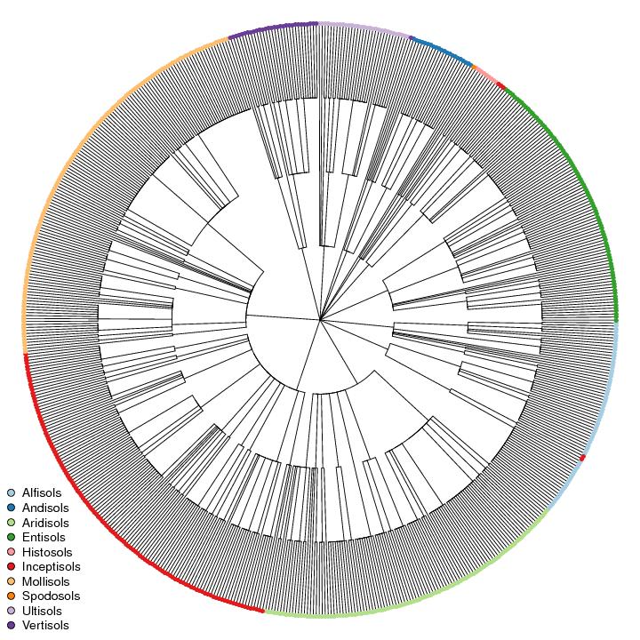
Figure: Subgroups from California
Implementation in R (source data is attached at the bottom of the page)
# need these
library(ape)
library(cluster)
library(RColorBrewer)

# read-in saved data
s <- read.csv('ca-data.csv')

# remove bad records that are missing data
s <- na.omit(s)

# inspect data
str(s)
'data.frame':   619 obs. of  4 variables:
 $ soilorder : Factor w/ 10 levels "Alfisols","Andisols",..: 1 1 1 1 1 1 1 1 1 1 ...
 $ suborder  : Factor w/ 50 levels "Albolls","Andepts",..: 3 3 3 3 3 3 3 3 3 3 ...
 $ greatgroup: Factor w/ 154 levels "Albaqualfs","Albaquults",..: 1 1 34 52 52 52 106 106 106 114 ...
 $ subgroup  : Factor w/ 573 levels "Abruptic Argiduridic Durixerolls",..: 263 339 366 265 382 461 15 182 420 14 ...

head(s)
  soilorder suborder  greatgroup            subgroup
1  Alfisols  Aqualfs  Albaqualfs   Mollic Albaqualfs
2  Alfisols  Aqualfs  Albaqualfs    Typic Albaqualfs
3  Alfisols  Aqualfs  Duraqualfs    Typic Duraqualfs
4  Alfisols  Aqualfs Endoaqualfs  Mollic Endoaqualfs
5  Alfisols  Aqualfs Endoaqualfs   Typic Endoaqualfs
6  Alfisols  Aqualfs Endoaqualfs Udollic Endoaqualfs


# perform clustering
# use divisive hierarchical clustering
d <- daisy(s)
d.h <- as.hclust(diana(d))
d.h$labels <- s$subgroup
p <- ladderize(as.phylo(d.h))

# setup colors for plotting, based on soil order
cols <- brewer.pal(n=length(unique(s$soilorder)), 'Paired')

# make the figure
plot.phylo(p, cex=0.5, font=1, type='fan', no.margin=TRUE, show.tip.label=FALSE)
tiplabels(pch=16, cex=1, col=cols[as.numeric(factor(s$soilorder))])
legend('bottomleft', legend=unique(s$soilorder), pt.bg=cols, pt.cex=1.5, pch=21, cex=1.15, bty='n')
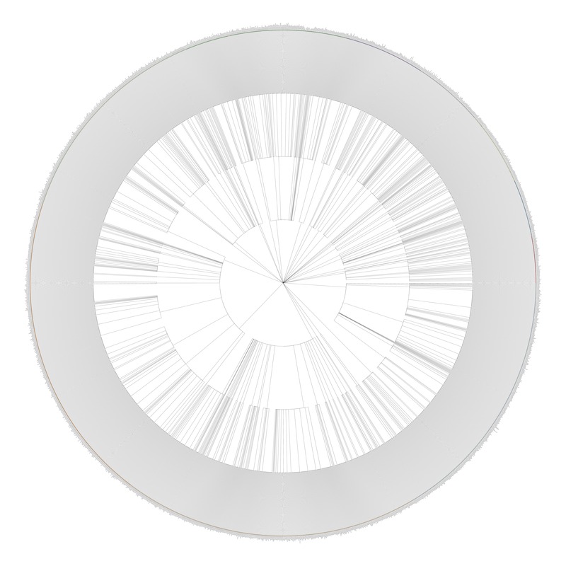
Figure: Subgroups from the lower 48 states
Attachment: ca-data.csv
