
 Premise
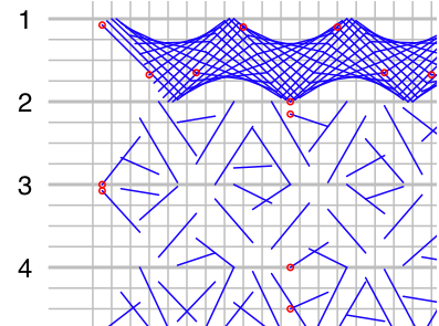
My wife asked me to come up with some graph paper for creating smocking patterns. After a couple of minutes playing around with R-base graphics functions, it occurred to me that several functions in the sp package would simplify grid-based operations. Some example functions, along with a simple approach to generating "interesting" patterns, are listed below.
Function Definitions
# make a nice grid from given grid topology
gg <- function(x)
{
# convert to spatial grid
x.sg <- SpatialGrid(x)

# extract grid axes
x.cv <- coordinatevalues(x)

# setup plot region
xy.min <- sapply(x.cv, min)
xy.max <- sapply(x.cv, max)

plot(1,1, cex=0.25, type='n', xlim=c(xy.min[1], xy.max[1]), ylim=c(xy.min[2], xy.max[2]), axes=FALSE)

# add grid
abline(h=x.cv$s2, v=x.cv$s1, col='grey', lty=1)
abline(h=seq(-0.5, max(x.cv$s2), by=4), col='grey', lty=1, lwd=2)

# make axis labels
y.axis.at <- seq(from=xy.max[2], to=xy.min[2], by=-4)
y.axis.lab <- seq(along=y.axis.at)
axis(side=2, at=y.axis.at, labels=y.axis.lab, lwd=NA, las=2, pos=-1)

# return grid information
return(list(xy.min=xy.min, xy.max=xy.max, offset=x@cellcentre.offset))
}

# plot a point on the grid
# referenced from the upper-left corner
# this function is vectorized, because points() is vectorized
gp <- function(x,y, grid.pars, ...)
{
x.prime <- x
y.prime <- (grid.pars$xy.max[2] - grid.pars$offset[2]) - (y - 1)
points(x.prime, y.prime, ...)
}

gs <- function(x.1, y.1, x.2, y.2, grid.pars, ...)
{
x.1.prime <- x.1
x.2.prime <- x.2
y.1.prime <- (grid.pars$xy.max[2] - grid.pars$offset[2]) - (y.1 - 1)
y.2.prime <- (grid.pars$xy.max[2] - grid.pars$offset[2]) - (y.2 - 1)
segments(x.1.prime, y.1.prime, x.2.prime, y.2.prime, ...)
}

# make something more interesting
gsin <- function(grid.pars, x_start, x_length, dx, x_lag, y_start, y_phase_i, y_phase_f, y_amp_i, y_amp_f, ...)
{
# generate x-coordinate sequence
x.i <- seq(x_start, x_length, by=dx)
x.f <- x.i + x_lag

# generate y-coordinate sequence
y.i <- round(y_start + sin(x.i + y_phase_i) * y_amp_i, 1)
y.f <- round(y_start + sin(x.f + y_phase_f) * y_amp_f,1 )

# plot segments
gs(x.i, y.i, x.f, y.f, grid.pars, ...)

# why not add a point at the strting point of every 10th stitch
gp(x.i[seq(along=x.i, by=10)], y.i[seq(along=x.i, by=10)], grid.pars, pch=1, cex=0.5, col='red')

# return segment information
return(list(x.i=x.i, y.i=y.i, x.f=x.f, y.f=y.f))
}
Example Application
library(sp)

# setup grid topology
x <- GridTopology(
cellcentre.offset=c(0.5,0.5),
cellsize=c(1,1),
cells.dim=c(60,40)
)


# init a new grid
grid.pars <- gg(x)

# neat design
gsin(grid.pars, 1, 55, .25, 4, 2.5, pi, pi, 2, 2, col='blue')
gsin(grid.pars, 1, 55, 1, 2, 6.5, pi/4, pi, 2, 2, col='blue')
gsin(grid.pars, 1, 55, 1, 2, 10.5, pi, 2*pi, 2, 2, col='blue')
gsin(grid.pars, 1, 55, 1, 2, 14.5, pi/2, pi, 2, 2, col='blue')
gsin(grid.pars, 1, 55, 1, 2, 19, pi, pi, 2, 0.5, col='blue')
gsin(grid.pars, 1, 55, 1, 0.5, 23.5, 2*pi, pi, 1, 1, col='blue')
gsin(grid.pars, 1, 55, 1, 0.5, 26.5, pi, pi, 1.5, 1.5, col='blue')
gsin(grid.pars, 1, 55, 0.5, 2, 30.5, pi/2, pi/2, 1, 2, col='blue')
gsin(grid.pars, 1, 55, .75, 3, 34.5, pi/2, 2*pi, 1, 1, col='blue')
gsin(grid.pars, 1, 55, .5, .25, 39, pi/4, pi/2, 0.5, 2, col='blue')
