
Premise
I was recently asked to print out a fabric pattern that could be used to cover a sphere, about the size of a ping pong ball, for the purposes of re-creating a favorite cat toy (quite important). Thinking this over, I realized that this was basically a map projection problem-- and could probably be solved by scaling an interrupted sinusoidal projection to match the geometry of a ping pong ball. Below are some R functions, and examples of how this endeavor evolved. Thanks to Greg Snow for this helpful post on the R-mailing list, describing how to preserve linear measurement when composing a figure in R. So far the pattern doesn't quite fit.
Update
It looks like it was not the printer's fault-- I had used the wrong radius for a ping pong ball: 16mm instead of 19mm or 20mm (there are 38mm and 40mm diameter ping pong balls). Updated files are attached.
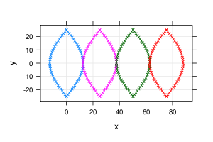
Figure: Sinusoidal Projection
Function Defs
# scale to C of ping pong ball:
# r = 16mm
# C = 2 * pi * 19  = 119.3805 mm (for a 38mm diameter ball)
# A = 4 * pi * r^2 = 4536.46 sq. mm

# n: number of slices
# circ: target circumference
# d: number of degrees per increment
sphere.slice <- function(n=4, circ, d=10)
        {

        # define sinusoidal projection function, fully vectorized
        # http://en.wikipedia.org/wiki/Sinusoidal_projection
        f <- function(lon, lat, lon_0=0, x_0=0)
                {
                x <- x_0 + ( (lon - lon_0) * cos((lat*pi/180)) )
                y <- lat
                d <- data.frame(x, y)
                return(d)
                }

        # temp lists used to store intermediate results
        l <- list()
        l.sin <- list()

        # sequences that define longitudinal slices:
        # slice edges
        s <- seq(from=-180, to=180, by=360/n)
        # slice centers
        s_lon_0 <- seq(from=-180, to=180, by=360/n) + (360/n)/2
        # slice false eastings
        s_x_0 <- seq(from=0, to=360, by=360/n)


        # generate slices
        for(i in 1:n)
                {
                l[[i]] <- rbind(data.frame(lon=s[i], lat=seq(-90, 90, by=d)), data.frame(lon=s[i+1], lat=seq(90, -90, by=-d)))
                }

        # project slices
        for(i in 1:n)
                {
                l.sin[[i]] <- data.frame(f(l[[i]]$lon, l[[i]]$lat, lon_0=s_lon_0[i], x_0=s_x_0[i]), lon_0=s_lon_0[i])
                }

        # combine into DF
        g <- ldply(l.sin)

        # scale to user-supplied circumference
        g.scaled <- with(g, data.frame(x=x * circ/360, y=y * circ/360, lon_0=lon_0))

        # done!
        return(g.scaled)
        }
Try With Ping Pong Ball Geometry
# need these
library(lattice)
library(plyr)
library(sp)

# try it out
g.scaled <- sphere.slice(n=4, circ=2*pi*19, d=5)

#check visually: aspect is scaled properly
xyplot(y ~ x, data=g.scaled, groups=lon_0, pch=4, cex=0.5, aspect='iso', type=c('p','g'))

## check circ: OK
sum(abs(range(g.scaled$x)))
sum(abs(range(g.scaled$y))) * 2

# check area, by converting to polygons
p.list <- by(g.scaled, g.scaled$lon_0, function(p) {
Polygon(round(p[,1:2], 4))
})

# compute total area of leaves
sum(sapply(p.list, function(i) i@area))

# this is only 3 sq.mm off
4533.58
Generate PDF Output at 1:1 Scale
## plot at 1:1 resolution for printing
# http://n4.nabble.com/plot-scale-td906260.html#a906260

# convert to inches
g.scaled.in <- with(g.scaled, data.frame(x=x * 0.03937008, y=y * 0.03937008, lon_0=lon_0))

dev.new()
tmp <- par('plt')
scale <- 1

dx <- diff(range(g.scaled.in$x))*1.08
wx <- grconvertX(dx/scale, from='inches', to='ndc')

dy <- diff(range(g.scaled.in$y))*1.08
wy <- grconvertY(dy/scale, from='inches', to='ndc')

par(plt = c(tmp[1], tmp[1]+wx, tmp[3], tmp[3]+wy) )

# setup plot, but don't actually plot anything
plot(g.scaled.in$x,g.scaled.in$y, type='n')

# add a grid
grid()

# add each slice, as lines
by(g.scaled.in, g.scaled.in$lon_0, function(i)
{
lines(i$x, i$y)
})
Attachment: sphere.pdf
