
A friend of mine recently published a very interesting article on the pedologic interpretation of asymetric peak functions fit to soil profile data (Myers et al., 2011). I won't bother summarizing or paraphrasing the article here, as the original article is very accessible, rather I thought I would share some new functionality in AQP that was inspired by the article. While reading the article I thought that it would be interesting to use one of these peak functions, the logistic power peak (LPP) function, to simulate soil property depth-functions. Simulated values could be used to evaluate new algorithms with a set of tightly controlled properties that vary with depth. One of the nice aspects of these peak functions is that they can create a wide range of shapes that mimic common anisotropic depth-functions associated with pedogenic processes such as illuviation, ferrolysis, or seasonal fluctuation of groundwater levels. An example R session demonstrating the use of LPP-simulated soil property depth-functions is presented below.
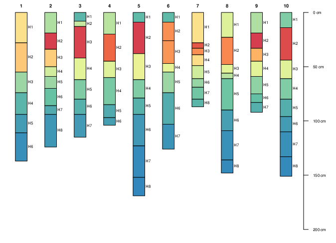
Image: LPP-simulated Profiles
Generate 10 Simulated Soil Profiles with fixed LPP Parameters
library(aqp)
require(RColorBrewer)
require(latticeExtra)

# read the manual page
?random_profile

# init some colors and a function to interpolate colors
cols <- rev(brewer.pal(8, 'Spectral'))
cr <- colorRamp(cols)

# make some simulated profiles with defined LPP parameters
d <- ldply(1:10, random_profile, n=c(6, 7, 8), n_prop=1, method='LPP',
lpp.a=5, lpp.b=10, lpp.d=5, lpp.e=5, lpp.u=25)

# color horizons based on simulated property
hz.cols <- cr(rescaler(d$p1, type='range'))
d$soil_color <- rgb(hz.cols, max=255)

# upgrade to SoilProfileCollection object
depths(d) <- id ~ top + bottom

# plot
plot(d)
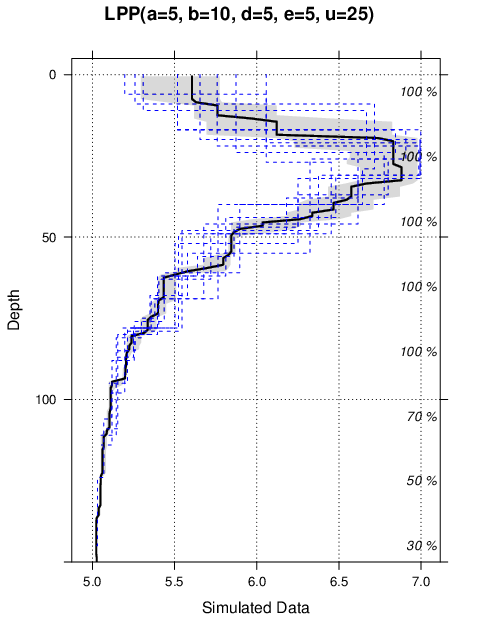
Image: Aggregate LPP-simulated Data
Plot the Original 10 Simulated Profiles, Along with slice-wise Median and IQR
# aggregated over all profiles, along 1cm-slices
a <- slab(d, fm= ~ p1)

# compute slice mid-points for plotting
a$mid <- with(a, (top + bottom) / 2)

# plot and save results for later...
(p1 <- xyplot(mid ~ p.q50, data=a,
lower=a$p.q25, upper=a$p.q75, ylim=c(150,-5), alpha=0.5,
panel=panel.depth_function, prepanel=prepanel.depth_function,
cf=a$contributing_fraction, xlab='Simulated Data', ylab='Depth',
main='LPP(a=5, b=10, d=5, e=5, u=25)',
par.settings=list(superpose.line=list(col='black', lwd=2))
))


# add original data as step-functions
p1 + as.layer(xyplot(top ~ p1, groups=id, data=horizons(d),
horizontal=TRUE, type='S',
par.settings=list(superpose.line=list(col='blue', lwd=1, lty=2))))
References
Myers, D.B., N.R. Kitchen, K.A. Sudduth, R.J. Miles, E.J. Sadler, and S. Grunwald. 2011. Peak Functions for Modeling High Resolution Soil Profile Data. Geoderma. 166(1): 74-83.
