
Premise
SSURGO is a digital, high-resolution (1:24,000), soil survey database produced by the USDA-NRCS. It is one of the largest and most complete spatial databases in the world; and is available for nearly the entire USA at no cost. These data are distributed as a combination of geographic and text data, representing soil map units and their associated properties. Unfortunately the text files do not come with column headers, so a template is required to make sense of the data. Alternatively, one can use an MS Access templateto attach column names, generate reports, and other such tasks. CSV file can be exported from the MS Access database for further use. A follow-up post with text file headers, and complete PostgreSQL database schema will contain details on implementing a SSURGO database without using MS Access.
If you happen to have some of the SSURGO tabular data that includes column names, the following R code may be of general interest for resolving the 1:many:many hierarchy of relationships required to make a thematic map.
This is the format we want the data to be in
    mukey     clay      silt      sand water_storage
   458581 20.93750 20.832237 20.861842     14.460000
   458584 43.11513 30.184868 26.700000     23.490000
   458593 50.00000 27.900000 22.100000     22.800000
   458595 34.04605 14.867763 11.776974     18.900000
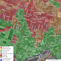
So we can make a map like this
Loading Data Into R
# need this for ddply()
library(plyr)

# load horizon and component data
chorizon <- read.csv('chorizon_table.csv')

# only keep some of the columns from the component table
component <- read.csv('component_table.csv')[,c('mukey','cokey','comppct_r')]
Function Definitions
# custom function for calculating a weighted mean
# values passed in should be vectors of equal length
wt_mean <- function(property, weights)
        {
        # compute thickness weighted mean, but only when we have enough data
        # in that case return NA

        # save indices of data that is there
        property.that.is.na <- which( is.na(property) )
                property.that.is.not.na <- which( !is.na(property) )

        if( length(property) - length(property.that.is.na) >= 1)
                prop.aggregated <- sum(weights[property.that.is.not.na] * property[property.that.is.not.na], na.rm=TRUE) / sum(weights[property.that.is.not.na], na.rm=TRUE)
        else
                prop.aggregated <- NA

        return(prop.aggregated)
        }

profile_total <- function(property, thickness)
        {
        # compute profile total
        # in that case return NA

        # save indices of data that is there
        property.that.is.na <- which( is.na(property) )
                property.that.is.not.na <- which( !is.na(property) )

        if( length(property) - length(property.that.is.na) >= 1)
                prop.aggregated <- sum(thickness[property.that.is.not.na] * property[property.that.is.not.na], na.rm=TRUE)
        else
                prop.aggregated <- NA

        return(prop.aggregated)
        }

# define a function to perfom hz-thickness weighted aggregtion
component_level_aggregation <- function(i)
        {

        # horizon thickness is our weighting vector
        hz_thick <- i$hzdepb_r - i$hzdept_r

        # compute wt.mean aggregate values
        clay <- wt_mean(i$claytotal_r, hz_thick)
        silt <- wt_mean(i$silttotal_r, hz_thick)
        sand <- wt_mean(i$sandtotal_r, hz_thick)
        # compute profile sum values
        water_storage <- profile_total(i$awc_r, hz_thick)

        # make a new dataframe out of the aggregate values
        d <- data.frame(cokey=unique(i$cokey), clay=clay, silt=silt, sand=sand, water_storage=water_storage)

        return(d)
        }

mapunit_level_aggregation <- function(i)
        {
        # component percentage is our weighting vector
        comppct <- i$comppct_r

        # wt. mean by component percent
        clay <- wt_mean(i$clay, comppct)
        silt <- wt_mean(i$silt, comppct)
        sand <- wt_mean(i$sand, comppct)
        water_storage <- wt_mean(i$water_storage, comppct)

        # make a new dataframe out of the aggregate values
        d <- data.frame(mukey=unique(i$mukey), clay=clay, silt=silt, sand=sand, water_storage=water_storage)

        return(d)
        }
Performing the Aggregation
# aggregate horizon data to the component level
chorizon.agg <- ddply(chorizon, .(cokey), .fun=component_level_aggregation, .progress='text')

# join up the aggregate chorizon data to the component table
comp.merged <- merge(component, chorizon.agg, by='cokey')

# aggregate component data to the map unit level
component.agg <- ddply(comp.merged, .(mukey), .fun=mapunit_level_aggregation, .progress='text')

# save data back to CSV
write.csv(component.agg, file='something.csv', row.names=FALSE)
Attachment:
Links:
Additive Time Series Decomposition in R: Soil Moisture and Temperature Data
R: advanced statistical package
Cluster Analysis 1: finding groups in a randomly generated 2-dimensional dataset
