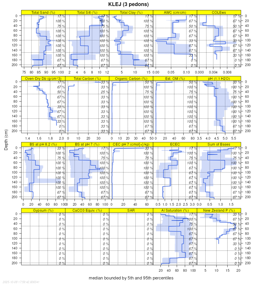
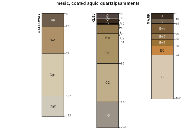
Aggregate lab data for the KLEJ soil series. This aggregation is based on all pedons with a current taxon name of KLEJ, and applied along 1-cm thick depth slices. Solid lines are the slice-wise median, bounded on either side by the interval defined by the slice-wise 5th and 95th percentiles. The median is the value that splits the data in half. Five percent of the data are less than the 5th percentile, and five percent of the data are greater than the 95th percentile. Values along the right hand side y-axis describe the proportion of pedon data that contribute to aggregate values at this depth. For example, a value of "90%" at 25cm means that 90% of the pedons correlated to KLEJ were used in the calculation. Source: KSSL snapshot (updated 2025-01-21). Methods used to assemble the KSSL snapshot used by SoilWeb / SDE
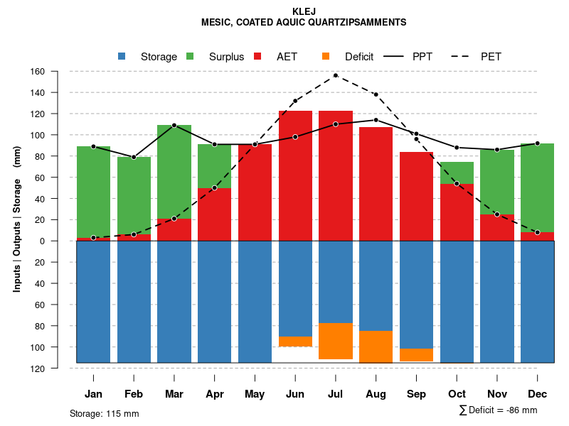
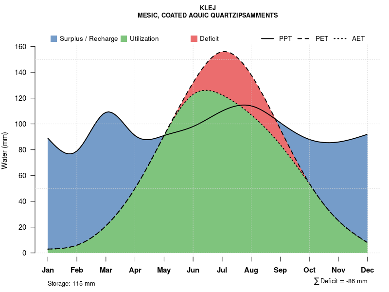
Monthly water balance estimated using a leaky-bucket style model for the KLEJ soil series. Monthly precipitation (PPT) and potential evapotranspiration (PET) have been estimated from the 50th percentile of gridded values (PRISM 1981-2010) overlapping with the extent of SSURGO map units containing each series as a major component. Monthly PET values were estimated using the method of Thornthwaite (1948). These (and other) climatic parameters are calculated with each SSURGO refresh and provided by the fetchOSD function of the soilDB package. Representative water storage values (“AWC” in the figures) were derived from SSURGO by taking the 50th percentile of profile-total water storage (sum[awc_r * horizon thickness]) for each soil series. Note that this representation of “water storage” is based on the average ability of most plants to extract soil water between 15 bar (“permanent wilting point”) and 1/3 bar (“field capacity”) matric potential. Soil moisture state can be roughly interpreted as “dry” when storage is depleted, “moist” when storage is between 0mm and AWC, and “wet” when there is a surplus. Clearly there are a lot of assumptions baked into this kind of monthly water balance. This is still a work in progress.
Click the image to view it full size.
Click the image to view it full size.
Sibling Summary
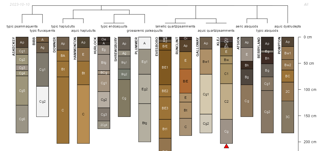
Siblings are those soil series that occur together in map units, in this case with the KLEJ series. Sketches are arranged according to their subgroup-level taxonomic structure. Source: SSURGO snapshot (updated 2025-10-03), parsed OSD records (updated 2026-01-02) and snapshot of SC database (updated 2026-01-02).
Click the image to view it full size.
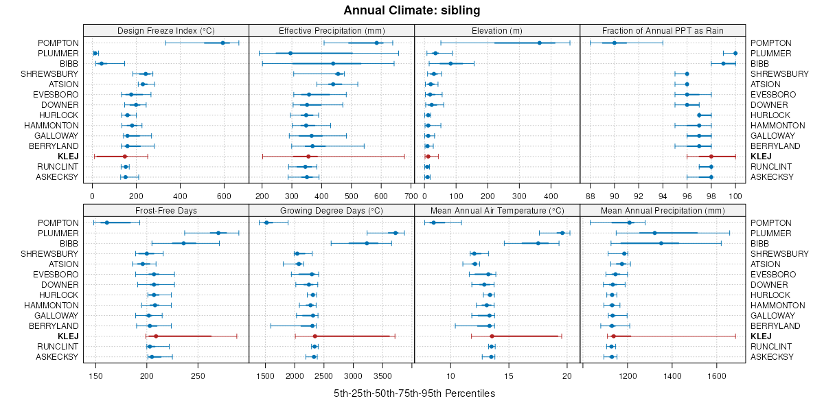
Select annual climate data summaries for the KLEJ series and siblings. Series are sorted according to hierarchical clustering of median values. Source: SSURGO map unit geometry and 1981-2010, 800m PRISM data (updated 2025-10-08).
Click the image to view it full size.
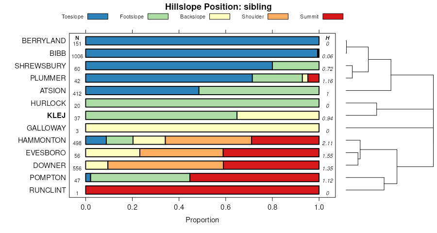
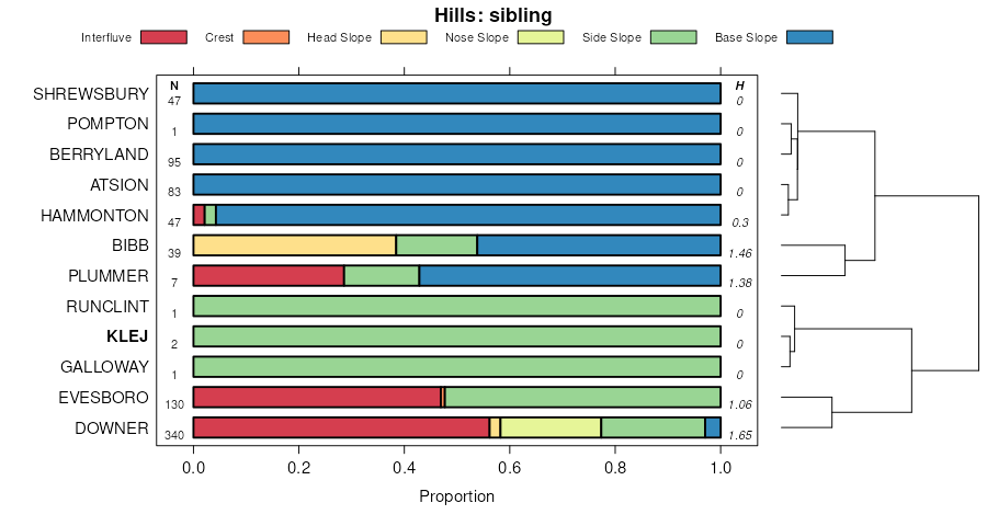
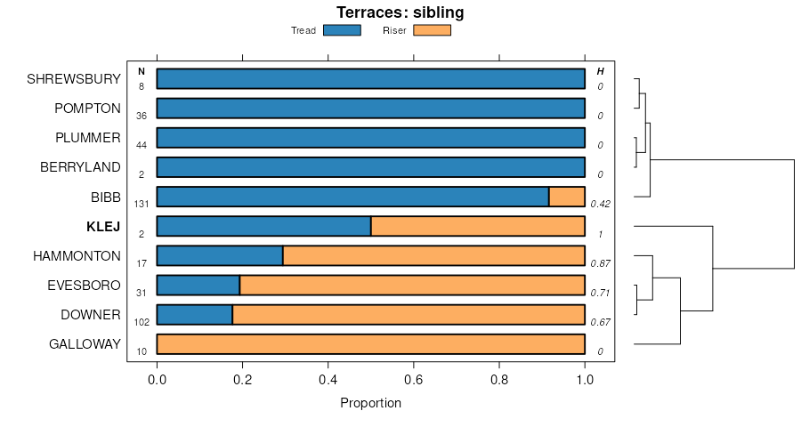
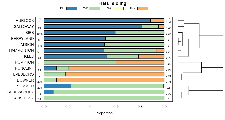
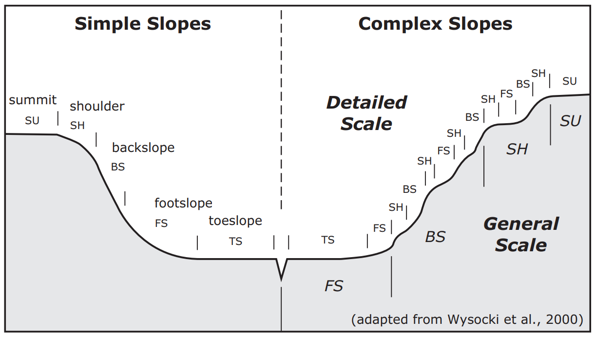
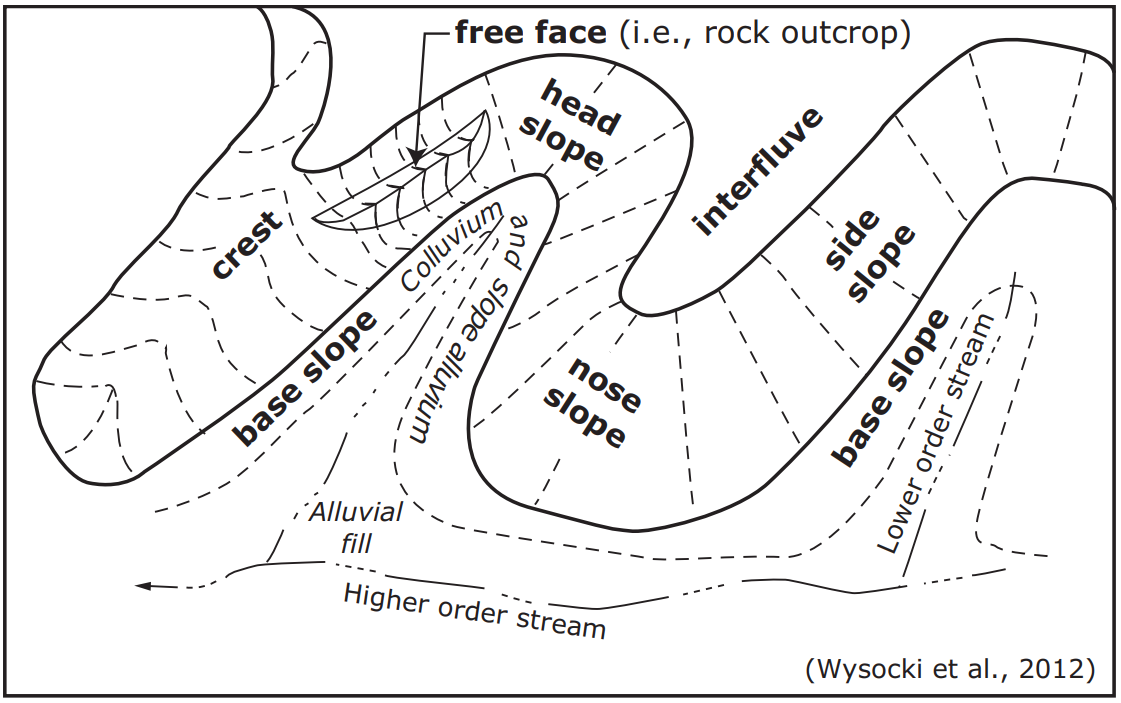
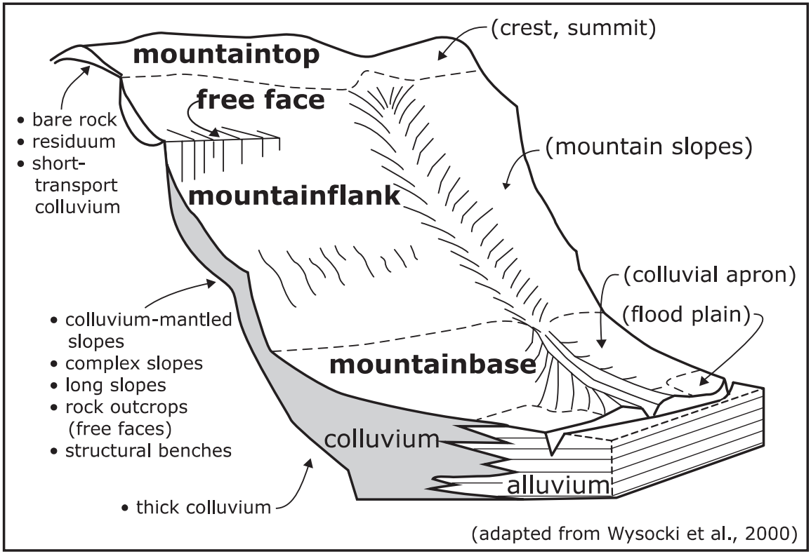
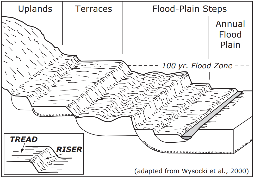
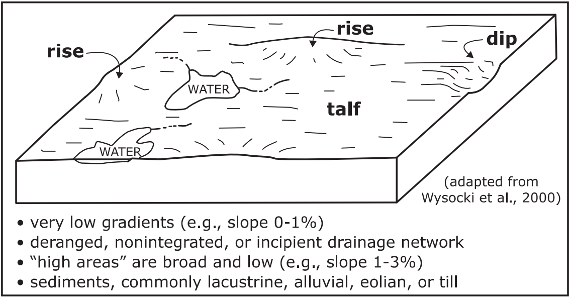
Geomorphic description summaries for the KLEJ series and siblings. Series are sorted according to hierarchical clustering of proportions and relative hydrologic position within an idealized landform (e.g. top to bottom).
Most soil series (SSURGO components) are associated with a hillslope position and one or more landform-specific positions: hills, mountain slopes, terraces, and/or flats.
Proportions can be interpreted as an aggregate representation of geomorphic membership. The values printed to the left (number of component records) and right (Shannon entropy) of stacked bars can be used to judge the reliability of trends. Small Shannon entropy values suggest relatively consistent geomorphic association, while larger values suggest lack thereof. Source: SSURGO component records (updated 2025-10-06).
Click the image to view it full size.
Click the image to view it full size.
There are insufficient data to create the 3D mountains figure.
Click the image to view it full size.
Click the image to view it full size.
Competing Series
Soil series competing with KLEJ share the same family level classification in Soil Taxonomy. Source: parsed OSD records (updated 2026-01-02) and snapshot of the SC database (updated 2026-01-02).
Click the image to view it full size.
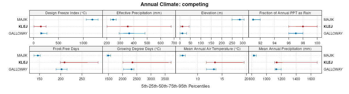
Select annual climate data summaries for the KLEJ series and competing. Series are sorted according to hierarchical clustering of median values. Source: SSURGO map unit geometry and 1981-2010, 800m PRISM data (updated 2025-10-08).
Click the image to view it full size.
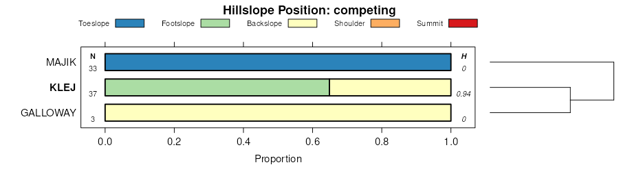
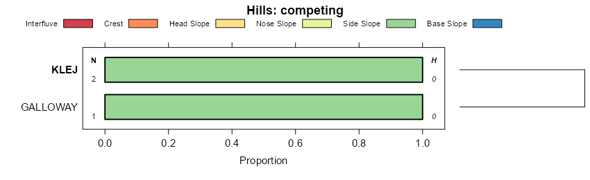
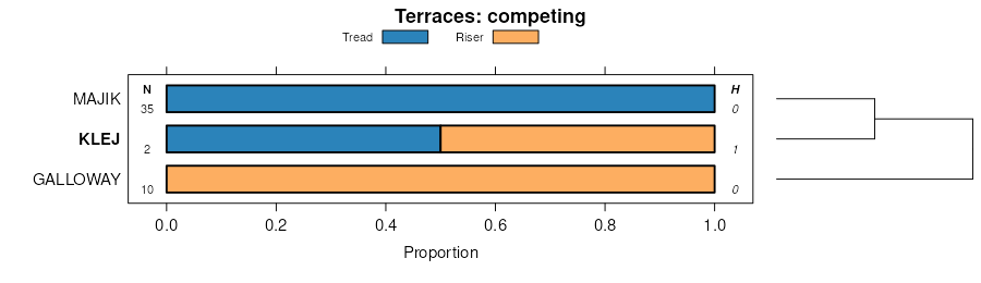
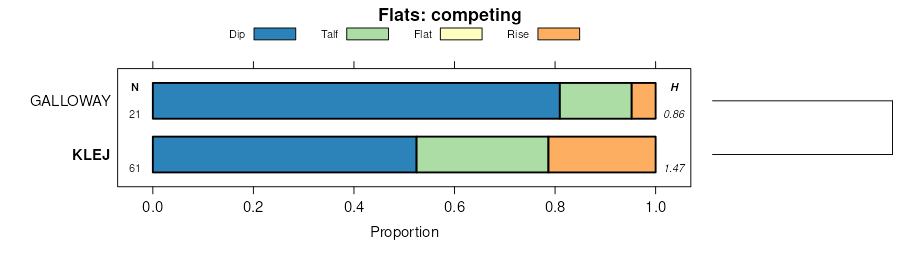
Geomorphic description summaries for the KLEJ series and competing. Series are sorted according to hierarchical clustering of proportions and relative hydrologic position within an idealized landform (e.g. top to bottom). Proportions can be interpreted as an aggregate representation of geomorphic membership.
Most soil series (SSURGO components) are associated with a hillslope position and one or more landform-specific positions: hills, mountain slopes, terraces, and/or flats.
The values printed to the left (number of component records) and right (Shannon entropy) of stacked bars can be used to judge the reliability of trends. Shannon entropy values close to 0 represent soil series with relatively consistent geomorphic association, while values close to 1 suggest lack thereof. Source: SSURGO component records (updated 2025-10-06).
Click the image to view it full size.
Click the image to view it full size.
There are insufficient data to create the 3D mountains figure.
Click the image to view it full size.
Click the image to view it full size.
Soil series sharing subgroup-level classification with KLEJ, arranged according to family differentiae. Hovering over a series name will print full classification and a small sketch from the OSD. Source: snapshot of SC database (updated 2026-01-02).
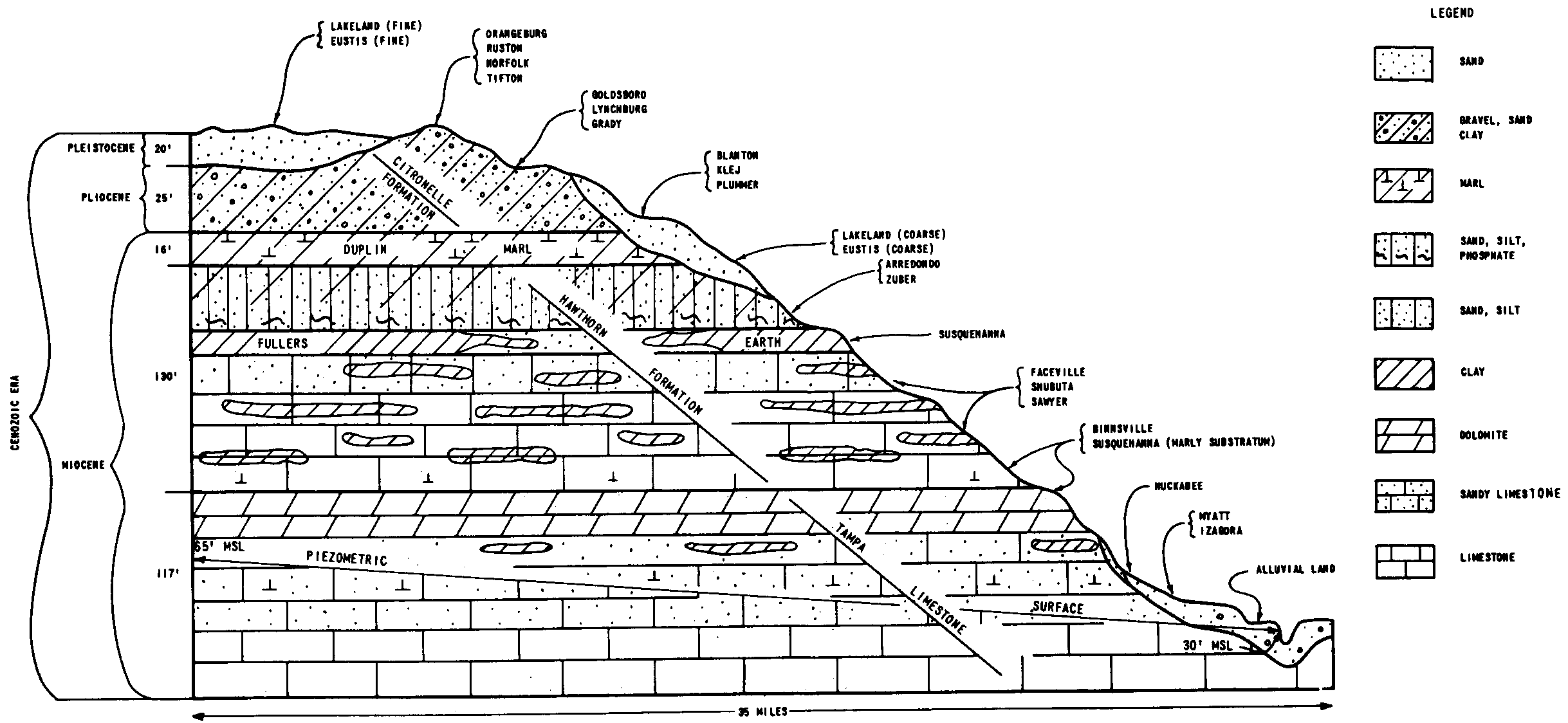
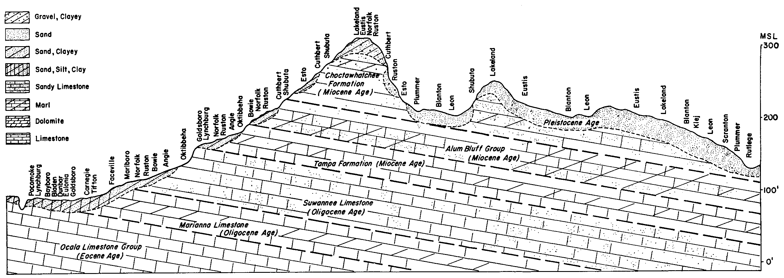
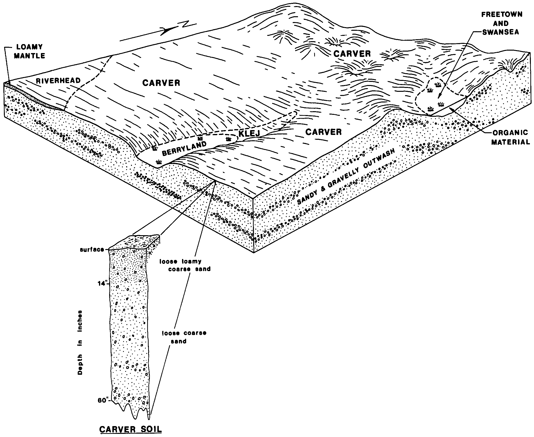
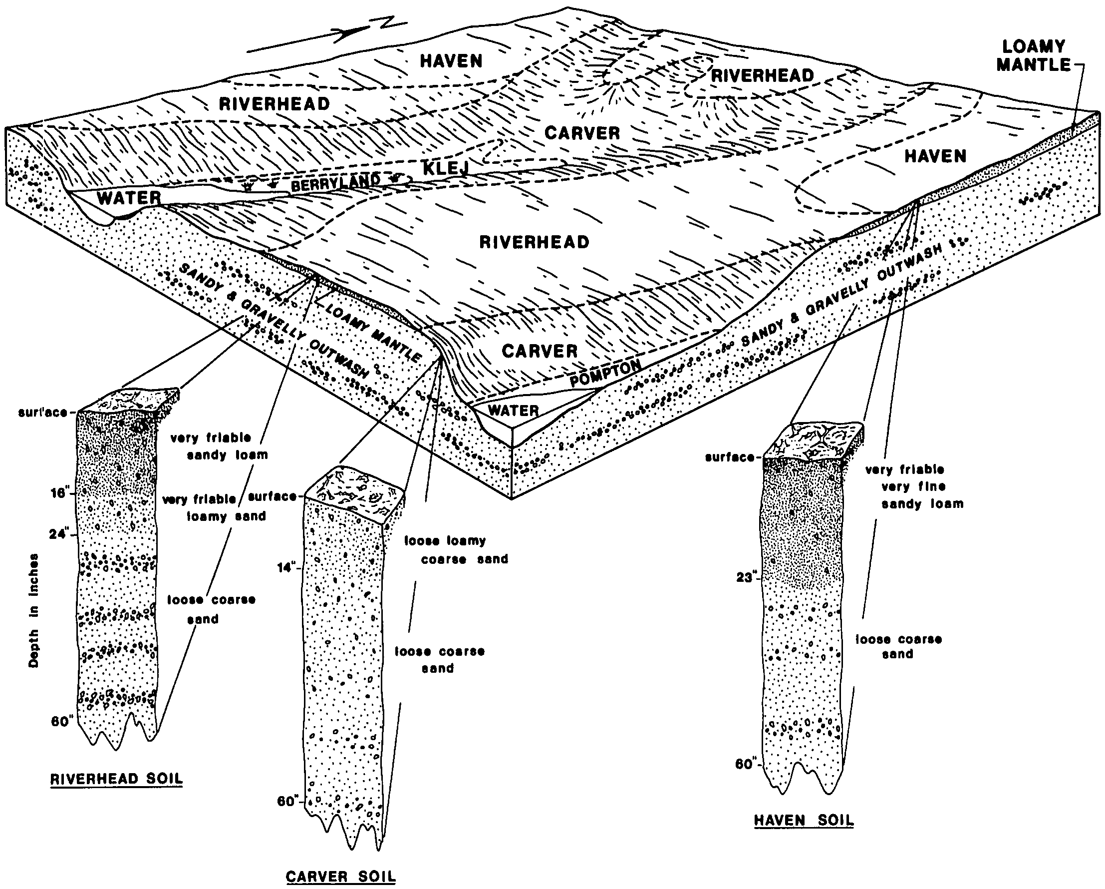
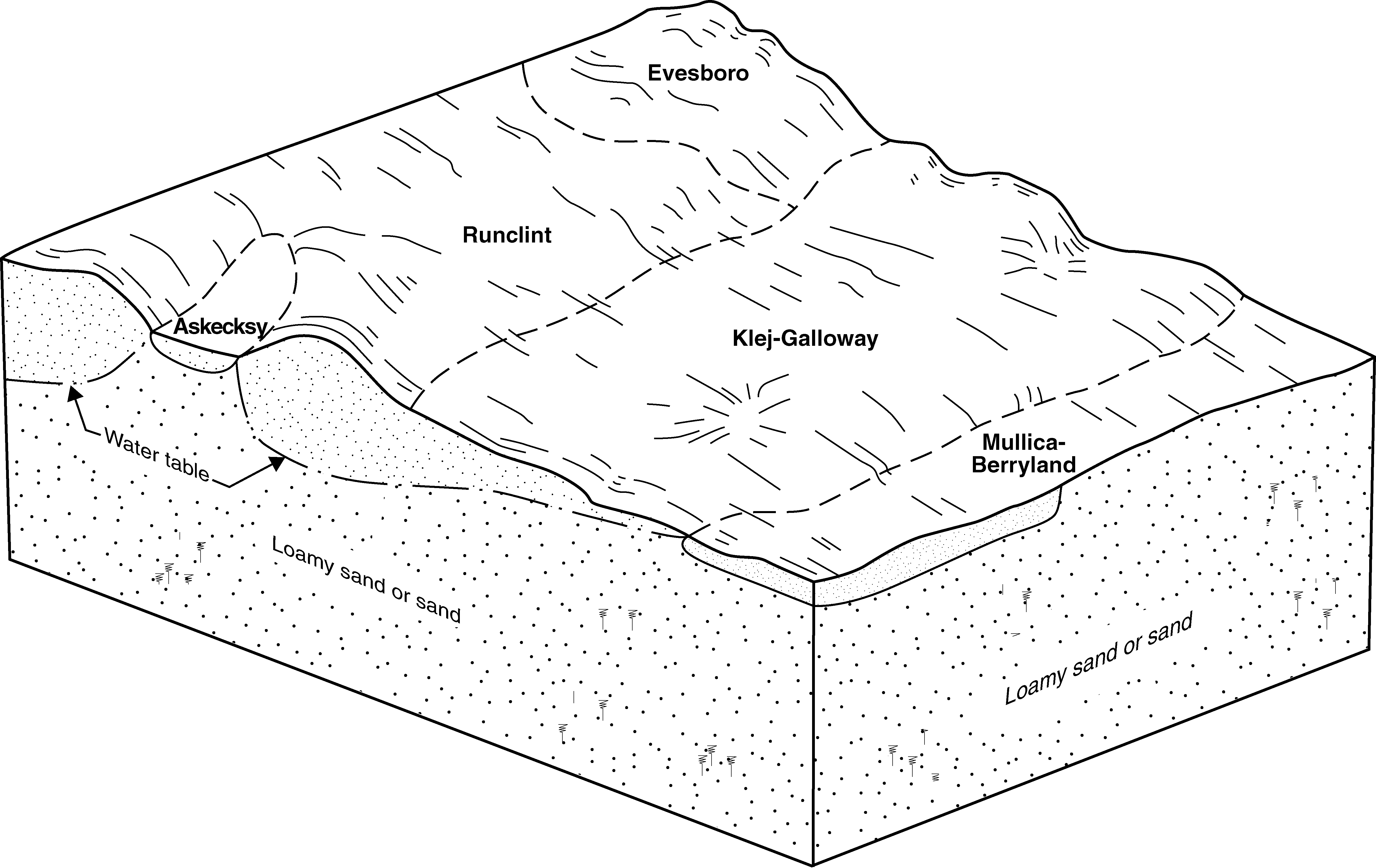
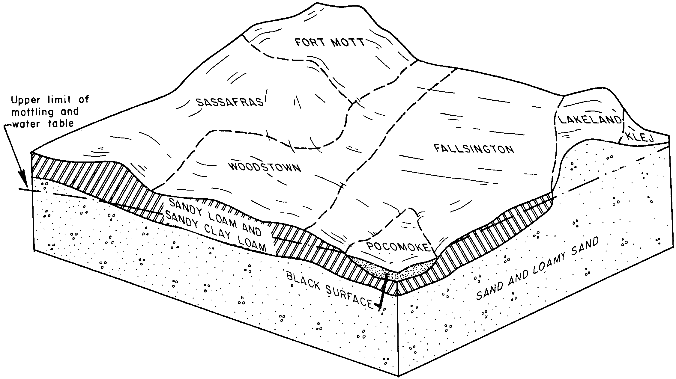
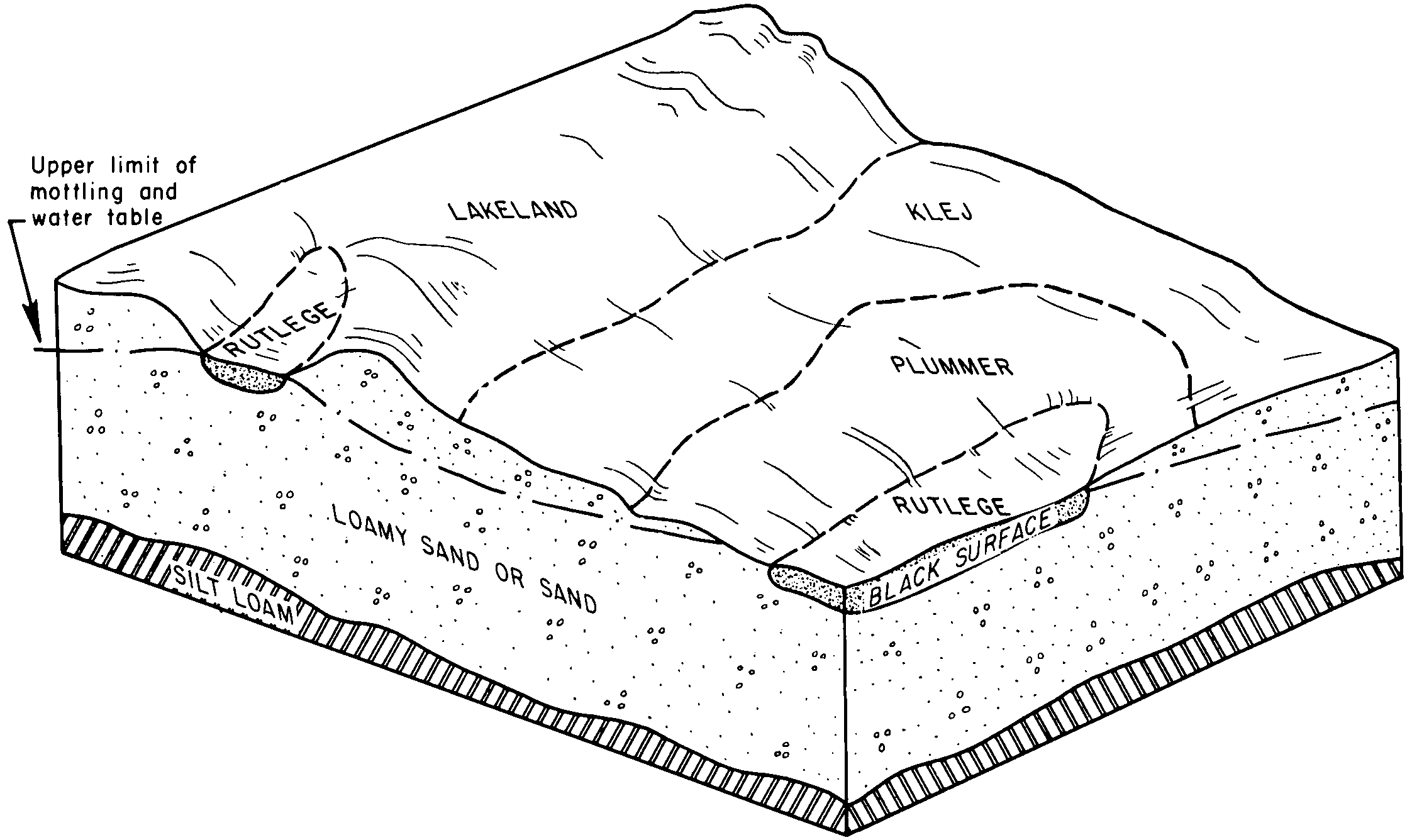
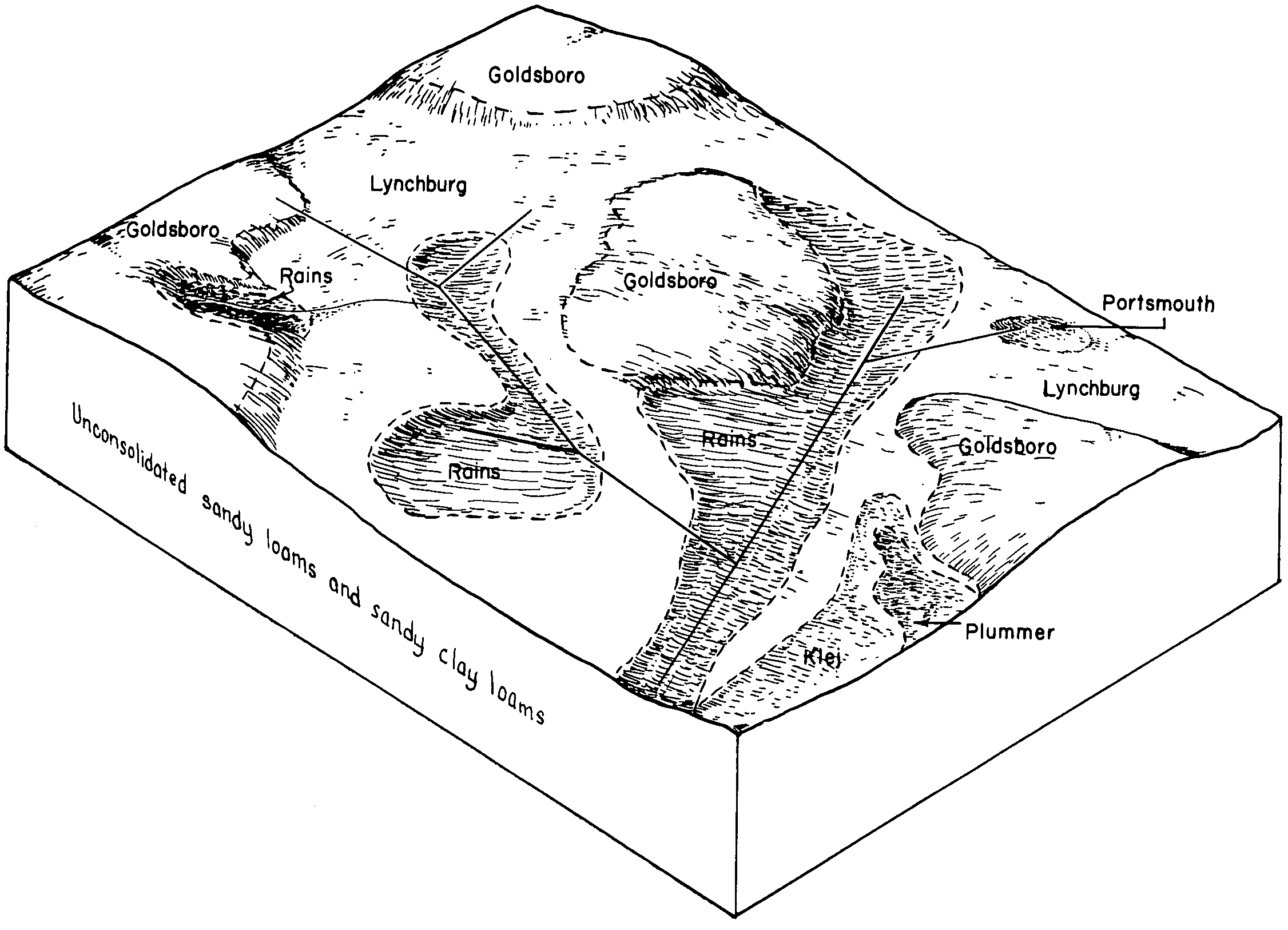
Block Diagrams
Click a link below to display the diagram. Note that these diagrams may be from multiple survey areas.
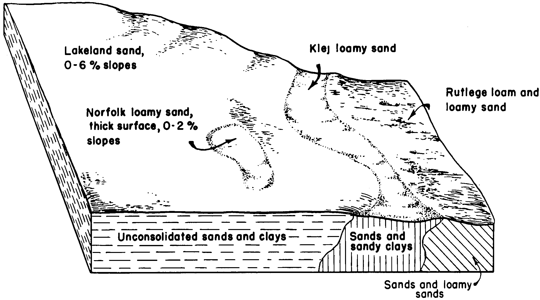
Typical pattern of soils and underlying material in the Riverhead-Carver-Haven general soil map unit (Soil Survey of Dukes County, Massachusetts; September 1986).
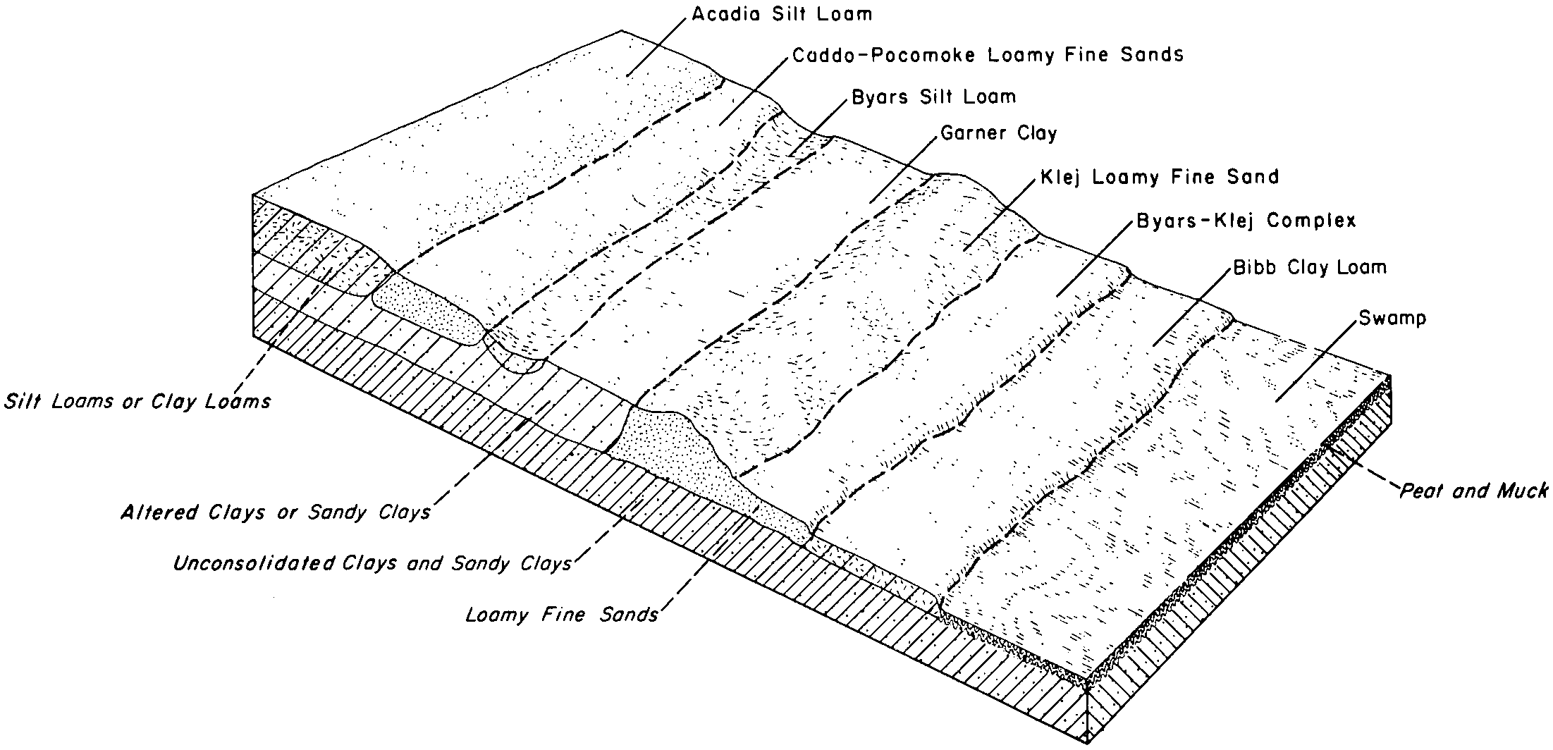
Cross section showing typical soil pattern in the Fallsington-Woodstown-Sassafras association (Soil Survey of Wicomico County, Maryland; January 1970).
Approximate geographic distribution of the KLEJ soil series. To learn more about how this distribution was mapped, or to compare this soil series extent to others, use the Series Extent Explorer (SEE) application.
Source: generalization of SSURGO geometry (updated 2025-10-04).