
I have mentioned the AQP package in previous entries. One of the functions in this package generates aggregate soil profile data, from a collection of soil profiles that are related by some factor: common lithology, common landscape position, and so on. Typically the mean, or median (50th percentile) is used to generate a new aggregate profile, that is representative of the original collection. Extending this idea, I thought that it would be interesting to generate aggregate profiles that are representative of the 25th and 75th percentiles as well. For the sake of clarity, lets call these three new profiles (25th, 50th, and 75th percentiles) Q25, Q50, and Q75. A 10 cm slicing interval was used as the basis upon which soil properties were aggregated.
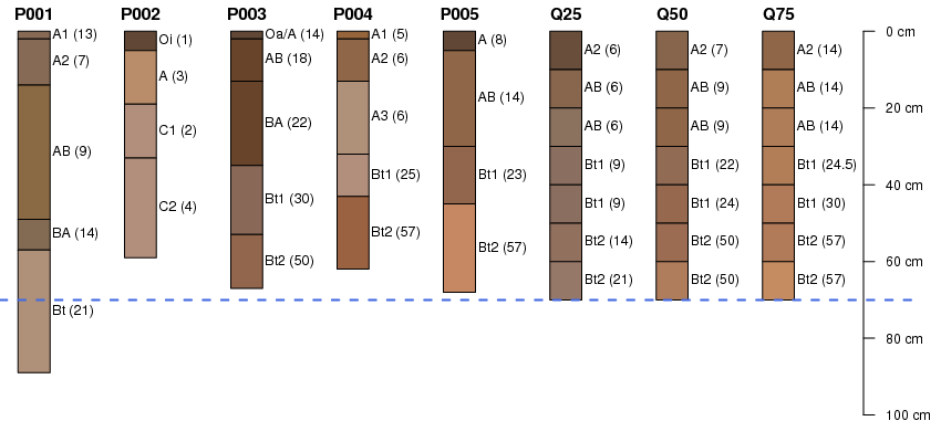
Using the soil profiles P001 - P005 (in the figure above), I generated the aggregate profiles Q25, Q50, and Q75 (see figure above). Horizon names are annotated, along with the clay content of each horizon in parenthesis. Soil colors are based on field-described, dry colors. The colors and clay contents of Q25 represent those values in the 25th percentile of the original collection: i.e. darker colors and lower clay contents. The horizon names assigned to Q25, Q50, and Q75 are based on the horizon name that was most common, within each depth slice. A blue line separates those slices within the aggregated profiles which were derived from at least 50% of the original collection. Slices below 70cm are excluded as they were only derived from P001. In most cases the median (Q50) aggregate profile would be the most useful description of the "central tendency" for a collection of soil profiles. Who knows, maybe it could be used in place of an official series description to describe a map unit. Or, it could be used within the context of a general soils map-- instead of listing all of the series within an aggregate map unit.
So that was interesting. Lets work on a different set of soil profile data, where we have measurements of clay content, CEC, and pH. What happens when we put the Q25, Q50, and Q75 aggregate profiles into a numerical profile classification alongside the original profiles? In other words, what if we numerically describe the pair-wise dissimilarity between all of the profiles in the collection, taking into account soil depth, several soil properties (clay content, CEC, pH), and how those properties vary with depth. The resulting dissimilarity matrix would describe the degree of similarity between any pair of soil profiles. Visualized as a dendrogram, it might look something like the following:
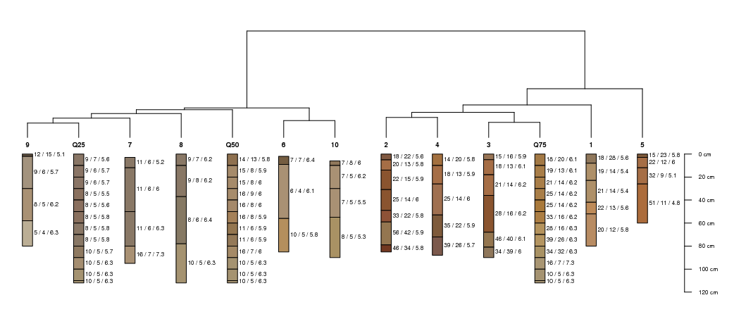
where the numerical dissimilarity between profiles is proportional to the height at which they are connected on the "tree". Horizon names illustrate clay content / CEC / pH. Note that the aggregate profiles have not been truncated according to the number of profiles contributing to their calculation-- and how this results in a fairly meaningless set of depth slices near the bottom of these profiles.
Alternatively, we could extract the pair-wise dissimilarity between each profile and the median profile (Q50). If we have adequately and unbiasedly sampled the landscape (a mighty large if!), this metric might tell us something about how much each profile deviates from the central tendency of soils within the sampled region. For the figure above, the normalized percent similarity between all profiles and Q50 is:
  1   2   3   4   5   6   7   8   9  10 Q25 Q75
 21   4  12  27   0  32  46  36  36  29  36  10
where profile "7" is the most similar to Q50. Interesting. Look for more examples like this within the AQP manual pages and vignette.
